Simulating data and power analysis for EFA

Simulation is the backbone of much of what we know about how exploratory factor analysis behaves: which retention criterion to trust, how large a sample a study needs, how badly non-normal or ordinal items distort a solution. EFAtools gives you two tools for this work. efa_simulate() draws data from a factor-model population you specify, with realistic departures from the ideal – model error, non-normal or ordinal marginals, missing values. efa_power() answers the sample-size question, either analytically from the RMSEA framework – which needs nothing but the model’s dimensions – or by Monte-Carlo simulation of the whole retain-and-fit pipeline on a population you specify.

library(EFAtools)

Throughout we use a three-factor population with six indicators per factor, taken from the shipped population_models data set (a collection of factor patterns and factor intercorrelation matrices used in simulation studies). All indicators load .6 on their factor, and the factors correlate .3.

Lambda <- population_models$loadings$baseline   # 18 indicators, 3 factors
Phi    <- population_models$phis_3$moderate      # factor correlations of .3

Simulating data with `efa_simulate()`

Specifying the population

A population can be given in one of two mutually exclusive ways: as the components of a factor model (Lambda, and optionally the factor intercorrelations Phi and the unique variances Psi), or as a ready population correlation matrix R. With the model components, the population correlation is assembled as $R = \Lambda \Phi \Lambda' + \Psi$ and standardized; when Psi is left unset it is filled in with the unique variances that make the population a correlation matrix.

sim <- efa_simulate(N = 500, Lambda = Lambda, Phi = Phi, seed = 42)
sim
#> Simulated data (<efa_simulated>)
#> 
#> 500 cases by 18 variables (continuous).
#> Marginals: normal.
#> 
#> Model error: none (exact population).

The drawn data sit in $data – here a 500-by-18 numeric matrix – and the population that was drawn from in $population.

dim(sim$data)
#> [1] 500  18
round(sim$population[1:6, 1:6], 2)
#>      V1   V2   V3   V4   V5   V6
#> V1 1.00 0.36 0.36 0.36 0.36 0.36
#> V2 0.36 1.00 0.36 0.36 0.36 0.36
#> V3 0.36 0.36 1.00 0.36 0.36 0.36
#> V4 0.36 0.36 0.36 1.00 0.36 0.36
#> V5 0.36 0.36 0.36 0.36 1.00 0.36
#> V6 0.36 0.36 0.36 0.36 0.36 1.00

If you only need the population correlation matrix – to inspect it, or to feed it back in as an R population – set return_pop = TRUE and no data are drawn:

R_pop <- efa_simulate(Lambda = Lambda, Phi = Phi, return_pop = TRUE)$population

# the same population can then be drawn from directly, via `R` instead of `Lambda`
sim_R <- efa_simulate(N = 500, R = R_pop, seed = 42)
dim(sim_R$data)
#> [1] 500  18

Model error: realistic misfit

A population assembled exactly from a factor model fits that model perfectly, which no real data set ever does. Simulating from an exact population therefore overstates how well factor-retention criteria and estimators recover the structure (MacCallum, 2003). To make a simulation realistic, efa_simulate() can perturb the population with model error so the factor model fits it only approximately, at a misfit you control through target_rmsea and/or target_cfi. Supplying a target is what switches model error on; the achieved fit is computed with the same formulas efa_fit() uses and returned in $model_error.

sim_me <- efa_simulate(N = 500, Lambda = Lambda, Phi = Phi,
                       target_rmsea = 0.05, seed = 42)
sim_me
#> Simulated data (<efa_simulated>)
#> 
#> 500 cases by 18 variables (continuous).
#> Marginals: normal.
#> 
#> Model error: CB
#> RMSEA: target .050, achieved .050
#> CFI: target --, achieved .936

Three methods are available through model_error. "CB" (Cudeck & Browne, 1992; the default) matches the target RMSEA to numerical precision and keeps the factor model the exact minimizer, so the CFI follows as a derived quantity:

c(rmsea = sim_me$model_error$rmsea, cfi = sim_me$model_error$cfi)
#>     rmsea       cfi 
#> 0.0500000 0.9363534

"TKL" (Tucker, Koopman, & Linn, 1969) adds minor common factors and is the only method that can target the CFI – on its own or, as here, together with the RMSEA, in which case it trades the two off:

efa_simulate(N = 500, Lambda = Lambda, Phi = Phi, model_error = "TKL",
             target_rmsea = 0.05, target_cfi = 0.95, seed = 42)$model_error[c("rmsea", "cfi")]
#> $rmsea
#> [1] 0.0455728
#> 
#> $cfi
#> [1] 0.9479115

"WB" (Wu & Browne, 2015) draws the population once from an inverse-Wishart distribution around the model-implied correlation. Being a single random draw, its realized RMSEA varies around the target (and tends to exceed it), so the value is reported rather than guaranteed:

efa_simulate(N = 500, Lambda = Lambda, Phi = Phi, model_error = "WB",
             target_rmsea = 0.05, seed = 42)$model_error$rmsea
#> [1] 0.06530353

Model error needs a factor-model population (there is no specified model to misfit against a bare R) with residual degrees of freedom and an exact factor structure (a diagonal Psi); it is orthogonal to the marginal, ordinal, and missing-data options below.

Non-normal marginals

By default the data are drawn with normal marginals. Real items – especially Likert-type ones – are rarely normal, and non-normality affects standard errors, fit indices, and the retention criteria. efa_simulate() can reproduce the population correlation while giving the variables non-normal marginals with a prescribed skewness and (excess) kurtosis, via two methods. marginals = "VM" is the Vale-Maurelli (1983) method:

sk <- function(x) mean(((x - mean(x)) / sd(x))^3)   # skewness of one column
sim_vm <- efa_simulate(N = 500, Lambda = Lambda, Phi = Phi, marginals = "VM",
                       skewness = 1.5, kurtosis = 4, seed = 42)
round(c(target = 1.5, achieved = mean(apply(sim_vm$data, 2, sk))), 2)
#>   target achieved 
#>     1.50     1.57

marginals = "IG" is the independent-generator method (Foldnes & Olsson, 2016), which covers non-normal distributions the Vale-Maurelli family cannot. Not every (skewness, kurtosis) pair is attainable – every distribution needs excess kurtosis of at least skewness^2 - 2, and each method covers a smaller region still – so an unreachable request is rejected with an informative error.

sim_ig <- efa_simulate(N = 500, Lambda = Lambda, Phi = Phi, marginals = "IG",
                       skewness = 1, kurtosis = 2, seed = 42)
round(c(target = 1, achieved = mean(apply(sim_ig$data, 2, sk))), 2)
#>   target achieved 
#>     1.00     0.96

A third option, marginals = "empirical", reproduces the population correlation while giving each variable the empirical marginal of a supplied data set (Ruscio & Kaczetow, 2008) – useful when you want your simulated variables to look exactly like real items. Only the marginals of marginal_data are used; its own correlations are ignored.

set.seed(123)
src <- matrix(rchisq(500 * nrow(Lambda), df = 3), ncol = nrow(Lambda))  # skewed source
sim_emp <- efa_simulate(N = 500, Lambda = Lambda, Phi = Phi,
                        marginals = "empirical", marginal_data = src, seed = 42)
# the drawn data inherit the shape of the source, not of a normal
round(c(source = mean(apply(src, 2, sk)),
        simulated = mean(apply(sim_emp$data, 2, sk))), 2)
#>    source simulated 
#>      1.60      1.58

Ordinal data

Setting categories discretizes the drawn data into ordered categories – the ordinal items of a typical questionnaire. Give it a single count (applied to every variable), one count per variable, or a list of category-proportion vectors. How the categorization relates to the population correlation is set by match.

With the default match = "thresholds", the data are cut at fixed thresholds on the standard-normal scale. Categorization attenuates product-moment correlations, so the categorized data’s Pearson correlation is smaller in magnitude than the population value:

sim_ord <- efa_simulate(N = 500, Lambda = Lambda, Phi = Phi, categories = 5, seed = 42)
# two indicators of the same factor: population vs. ordinal Pearson correlation
round(c(population = sim_ord$population[1, 2],
        ordinal    = cor(sim_ord$data)[1, 2]), 3)
#> population    ordinal 
#>      0.360      0.245

match = "polychoric" instead requires the latent to be normal, which is exactly the condition under which the polychoric correlation of the categorized data equals the target correlation. That is the guarantee you want when the downstream analysis will use polychoric correlations (efa_fit(..., cor_method = "poly")), because the estimated correlation matrix then targets the true population rather than the attenuated one. Because the guarantee rests on normality, the mode refuses to combine with the non-normal marginals above – which is the point of asking for it: under marginals = "normal" the draw itself is the same one "thresholds" makes, so what you gain is the check, not a different sampler.

sim_poly <- efa_simulate(N = 500, Lambda = Lambda, Phi = Phi, categories = 5,
                         match = "polychoric", seed = 42)
head(sim_poly$data[, 1:6])
#>      V1 V2 V3 V4 V5 V6
#> [1,]  3  5  4  4  4  5
#> [2,]  1  2  2  5  2  1
#> [3,]  2  1  4  1  3  4
#> [4,]  3  5  5  4  5  5
#> [5,]  2  2  3  3  2  1
#> [6,]  4  4  2  4  3  3

The recovery is a statement about the population polychoric, so it shows up in a single sample only up to sampling error: at N = 500 an individual polychoric estimate still scatters noticeably around the population value, while the Pearson correlation above is biased low no matter how large the sample grows.

At small N or with many categories a draw can leave a category empty, which destabilizes the polychoric correlation; efa_simulate() warns when that happens, so keep N comfortably large for the number of categories requested.

Missing data

missing imposes a missing-data mechanism (Rubin, 1976) on the drawn data, holing each variable at an expected rate missing_prop. "MCAR" masks values completely at random:

sim_mcar <- efa_simulate(N = 500, Lambda = Lambda, Phi = Phi,
                         missing = "MCAR", missing_prop = 0.1, seed = 42)
round(colMeans(is.na(sim_mcar$data))[1:6], 3)
#>    V1    V2    V3    V4    V5    V6 
#> 0.104 0.104 0.120 0.100 0.098 0.102

"MAR" makes each variable’s missingness depend on another variable, and "MNAR" on the variable’s own value, both through a logistic model whose slope is set by missing_strength. The realized rate of a given draw varies around the target.

sim_mar  <- efa_simulate(N = 500, Lambda = Lambda, Phi = Phi, missing = "MAR",
                         missing_prop = 0.15, seed = 42)
sim_mnar <- efa_simulate(N = 500, Lambda = Lambda, Phi = Phi, missing = "MNAR",
                         missing_prop = 0.15, missing_strength = 1.5, seed = 42)
round(c(MAR = mean(colMeans(is.na(sim_mar$data))),
        MNAR = mean(colMeans(is.na(sim_mnar$data)))), 3)
#>   MAR  MNAR 
#> 0.149 0.149

The returned matrix carries the NAs, which the correlation estimators (pairwise deletion, FIML, and so on) handle downstream. See the Ordinal and missing data vignette for analysing such data.

Several datasets and reproducibility

For a simulation study you need many datasets from the same population. Set n_datasets and $data becomes a list:

sims <- efa_simulate(N = 300, Lambda = Lambda, Phi = Phi, n_datasets = 5, seed = 42)
length(sims$data)
#> [1] 5
dim(sims$data[[1]])
#> [1] 300  18

Replicated draws are dispatched across replicates with future.apply, so selecting a parallel plan with future::plan() runs them in parallel; the default plan is sequential. A fixed seed assigns each replicate its own reproducible random-number stream, so the output is identical no matter how many workers run it – and the same call twice gives byte-identical data:

a <- efa_simulate(N = 300, Lambda = Lambda, Phi = Phi, seed = 42)
b <- efa_simulate(N = 300, Lambda = Lambda, Phi = Phi, seed = 42)
identical(a$data, b$data)
#> [1] TRUE

The seed is also restored afterwards, so the call leaves your own random-number stream untouched.

Power analysis with `efa_power()`

Analytic RMSEA power

The fastest power analysis needs no simulation at all. efa_power() (in its default mode = "rmsea") implements the RMSEA power framework of MacCallum, Browne, and Sugawara (1996), which refers the fit statistic to a noncentral chi-square distribution. Two tests are available. Under the test of close fit, the null hypothesis is that the fit is close (RMSEA ≤ eps0, conventionally .05), and power is the probability of rejecting that null when the true fit is worse (eps1, conventionally .08) – that is, the probability of detecting a model that is not close. The test of not-close fit reverses the logic: its null is that the fit is not close (RMSEA ≥ eps0), tested against a better alternative (eps1, conventionally .01).

Give a sample size to get the power at it. The model can be described either by its degrees of freedom directly or by its dimensions – here our 18-indicator, three-factor model:

efa_power(p = 18, k = 3, N = 200)
#> 
#> ── RMSEA power analysis ────────────────────────────────────────────────────────
#> 
#> Test of close fit: H0 RMSEA ≤ .050 vs. H1 RMSEA = .080.
#> alpha = .050 · df = 102
#> 
#> Power = .958 at N = 200.
#> Critical value χ²(102) = 187.289 · noncentrality H0 = 50.745, H1 = 129.907.

Leave N unset and give a target power instead to solve for the smallest sample size that reaches it:

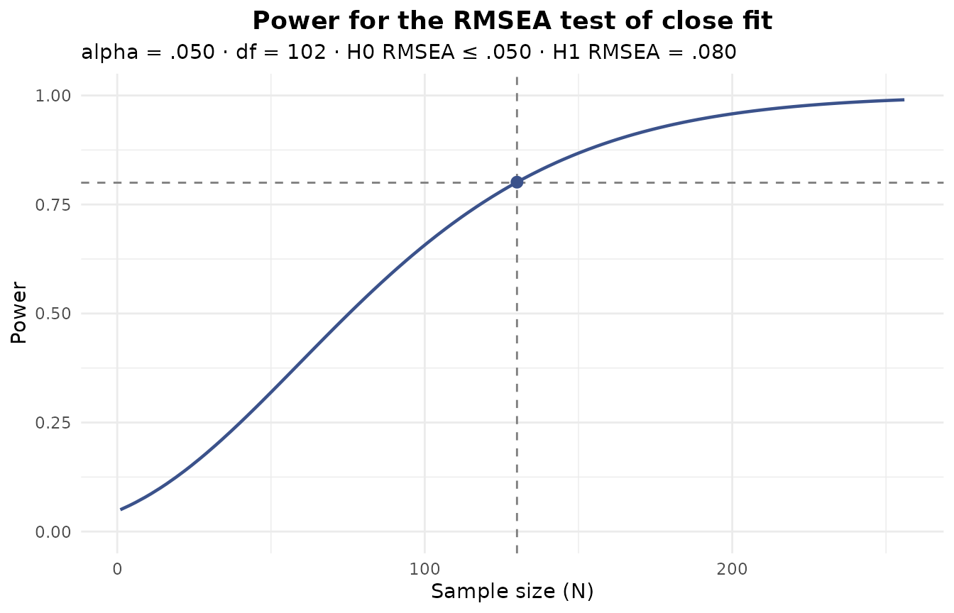
efa_power(p = 18, k = 3, power = 0.80)
#> 
#> ── RMSEA power analysis ────────────────────────────────────────────────────────
#> 
#> Test of close fit: H0 RMSEA ≤ .050 vs. H1 RMSEA = .080.
#> alpha = .050 · df = 102
#> 
#> Required N = 130 for a power of .800 (achieved .801).
#> Critical value χ²(102) = 166.326 · noncentrality H0 = 32.895, H1 = 84.211.

The test of not-close fit is selected with type (never by the ordering of eps0/eps1):

efa_power(p = 18, k = 3, N = 200, type = "notclose")
#> 
#> ── RMSEA power analysis ────────────────────────────────────────────────────────
#> 
#> Test of not-close fit: H0 RMSEA ≥ .050 vs. H1 RMSEA = .010.
#> alpha = .050 · df = 102
#> 
#> Power = .876 at N = 200.
#> Critical value χ²(102) = 121.042 · noncentrality H0 = 50.745, H1 = 2.030.

For a multiple-group model, group divides the noncentrality across groups. The reported N is the total across groups – 259 in all, about 130 per group – and N_per_group carries that per-group figure:

pw_2g <- efa_power(p = 18, k = 3, power = 0.80, group = 2)
pw_2g
#> 
#> ── RMSEA power analysis ────────────────────────────────────────────────────────
#> 
#> Test of close fit: H0 RMSEA ≤ .050 vs. H1 RMSEA = .080.
#> alpha = .050 · df = 102 · groups = 2
#> 
#> Required N = 259 (total; 129.5 per group) for a power of .800 (achieved .801).
#> Critical value χ²(102) = 166.326 · noncentrality H0 = 32.895, H1 = 84.211.
pw_2g$N_per_group
#> [1] 129.5

The plot() method draws power against sample size, marking the object’s own result. When a sample size was solved for, it marks the target power and the required N:

pw <- efa_power(p = 18, k = 3, power = 0.80)
plot(pw)

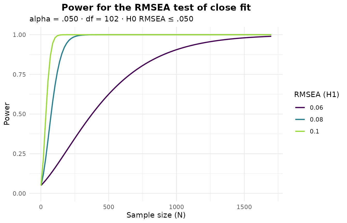
Sweeping the alternative RMSEA (or the degrees of freedom) overlays several curves, which is a compact way to see how the required sample size trades off against the effect you want to detect:

plot(pw, eps1 = c(0.06, 0.08, 0.10))

Simulation-based power

The analytic power above is about a fit statistic. Often the real question is different: how often will my factor-retention criteria point to the right number of factors, and how well will the fitted loadings recover the true pattern, at a given sample size? That needs a Monte-Carlo study of the whole pipeline, which is what mode = "simulation" runs. It draws n_datasets samples from the population (via efa_simulate()) and, over the replicates, reports three things: the hit-rate of each retention criterion (how often it recovers the true factor count), structure recovery (how often the fitted loadings match the population pattern by Tucker congruence), and the convergence and Heywood-case rate of the fit.

By default the population fits the model exactly, which – as in efa_simulate() – is optimistic. The printed summary says so:

efa_power("simulation", Lambda = Lambda, Phi = Phi, N = 300,
          n_datasets = 200, criteria = c("ekc", "map"), seed = 42)
#> 
#> ── EFA power simulation ────────────────────────────────────────────────────────
#> 
#> 18 variables · 3 factors · N = 300 · 200 datasets
#> Estimation: PAF · rotation: promax
#> Model error: none. The population is exact, so the hit-rate and recovery are
#> optimistic; set `target_rmsea` for realism.
#> 
#> Retention hit-rate P(k-hat = 3)
#> • EKC_BvA2017: .995 (n = 200)
#> • MAP_TR2: 1.000 (n = 200)
#> • MAP_TR4: 1.000 (n = 200)
#> 
#> Structure recovery (Tucker congruence ≥ .950)
#> • recovery rate (min congruence): 1.000 (n = 200)
#> • recovery rate (mean congruence): 1.000 (n = 200)
#> • median min congruence: .986
#> 
#> Convergence
#> • fits completed: 1.000 (200/200)
#> • converged (of completed): 1.000
#> • Heywood cases (of completed): .000

Supplying a misfit target makes the study realistic. In simulation mode a target on its own activates model error with the "TKL" method by default (it degrades both the hit-rate and recovery in a realistic way, unlike "CB", which keeps the fitted loadings the exact minimizer):

efa_power("simulation", Lambda = Lambda, Phi = Phi, N = 300,
          n_datasets = 200, criteria = c("ekc", "map"),
          target_rmsea = 0.05, seed = 42)
#> 
#> ── EFA power simulation ────────────────────────────────────────────────────────
#> 
#> 18 variables · 3 factors · N = 300 · 200 datasets
#> Estimation: PAF · rotation: promax
#> Model error (TKL): RMSEA = .050 · CFI = .936
#> 
#> Retention hit-rate P(k-hat = 3)
#> • EKC_BvA2017: .385 (n = 200)
#> • MAP_TR2: 1.000 (n = 200)
#> • MAP_TR4: .970 (n = 200)
#> 
#> Structure recovery (Tucker congruence ≥ .950)
#> • recovery rate (min congruence): .995 (n = 200)
#> • recovery rate (mean congruence): 1.000 (n = 200)
#> • median min congruence: .982
#> 
#> Convergence
#> • fits completed: 1.000 (200/200)
#> • converged (of completed): 1.000
#> • Heywood cases (of completed): .000

A few things to read off the output. The hit-rate is reported per criterion, and per variant where a criterion has several (the minimum-average-partial test reports its squared and fourth-power variants, for example); its denominator is the number of replicates on which the criterion returned a definite count, so a criterion that errored or was undecided on some replicates is not silently penalised. Structure recovery is available only for a factor-model population (a bare R carries no loadings to recover); a replicate counts as recovered when its matched-factor Tucker congruence reaches recovery_threshold, which defaults to the .95 that Lorenzo-Seva and ten Berge (2006) read as factors that can be considered equal. Here the strong .6 loadings make recovery near-perfect even under model error, while the criteria disagree markedly – exactly the kind of finding a power study exists to surface.

On the number of datasets. We use n_datasets = 200 here purely so the article builds quickly. A real power study should use the default of 500, and preferably more, to pin the rates down. We also evaluate only the two fastest criteria, "EKC" and "MAP"; the criteria that run their own internal simulation on every replicate – comparison data ("CD"), the hull method ("HULL"), the next-eigenvalue sufficiency test ("NEST"), and parallel analysis ("PARALLEL") – multiply the cost substantially. As in efa_simulate(), a seed makes the whole study reproducible and independent of the number of parallel workers.

Where to next

efa_simulate() and efa_power() carry more options than shown here – per-variable moments, category proportions, MAR predictors, the choice of estimator and rotation for the recovery fit. See ?efa_simulate and ?efa_power for the full argument lists and the structure of the returned objects, the EFAtools vignette for the analysis workflow these studies evaluate, and the Ordinal and missing data vignette for fitting the ordinal and incomplete data simulated above.

References

Cudeck, R., & Browne, M. W. (1992). Constructing a covariance matrix that yields a specified minimizer and a specified minimum discrepancy function value. Psychometrika, 57, 357-369.

Foldnes, N., & Olsson, U. H. (2016). A simple simulation technique for nonnormal data with prespecified skewness, kurtosis, and covariance matrix. Multivariate Behavioral Research, 51, 207-219.

Lorenzo-Seva, U., & ten Berge, J. M. F. (2006). Tucker’s congruence coefficient as a meaningful index of factor similarity. Methodology, 2, 57-64.

MacCallum, R. C. (2003). Working with imperfect models. Multivariate Behavioral Research, 38, 113-139.

MacCallum, R. C., Browne, M. W., & Sugawara, H. M. (1996). Power analysis and determination of sample size for covariance structure modeling. Psychological Methods, 1, 130-149.

Rubin, D. B. (1976). Inference and missing data. Biometrika, 63, 581-592.

Ruscio, J., & Kaczetow, W. (2008). Simulating multivariate nonnormal data using an iterative algorithm. Multivariate Behavioral Research, 43, 355-381.

Tucker, L. R., Koopman, R. F., & Linn, R. L. (1969). Evaluation of factor analytic research procedures by means of simulated correlation matrices. Psychometrika, 34, 421-459.

Vale, C. D., & Maurelli, V. A. (1983). Simulating multivariate nonnormal distributions. Psychometrika, 48, 465-471.

Wu, H., & Browne, M. W. (2015). Quantifying adventitious error in a covariance structure as a random effect. Psychometrika, 80, 571-600.

Simulating data with efa_simulate()

References

Cario, M. C., & Nelson, B. L. (1997). Modeling and generating random vectors with arbitrary marginal distributions and correlation matrix (Technical report). Department of Industrial Engineering and Management Sciences, Northwestern University.