EFA with ordinal and missing data
Source:vignettes/Ordinal_and_missing_data.Rmd
Ordinal_and_missing_data.RmdTwo features of real data complicate an exploratory factor analysis:
items are often ordinal (a handful of Likert categories
rather than a continuous scale), and some responses are usually
missing. EFAtools handles both within the
ordinary efa_fit() workflow, without switching packages.
This vignette shows how. It assumes familiarity with the basic workflow
covered in the EFAtools vignette and focuses
on what changes for ordinal and incomplete data.
So that the examples are self-contained and reproducible, we generate
the data with efa_simulate() from a known three-factor
population (18 indicators, six per factor, with moderately correlated
factors), using fixed seeds throughout.
Lambda <- population_models$loadings$baseline  # 18 x 3 loading pattern
Phi    <- population_models$phis_3$moderate    # moderate factor intercorrelations
Ordinal Data
Rating-scale items are not continuous: they take a few ordered values, and a Pearson correlation between two such items underestimates the association between the underlying constructs. The polychoric correlation instead estimates the correlation of the continuous latent variables assumed to underlie the observed categories, and pairing it with a categorical estimator removes the bias that treating the items as continuous introduces.
We draw 400 responses on a four-category scale. Because the latent
data are normal, cutting them at the standard-normal category thresholds
already leaves the population polychoric correlation of the
discretised data equal to the target correlation;
match = "polychoric" records that this is what we are
after.
d_ord <- efa_simulate(N = 400, Lambda = Lambda, Phi = Phi,
                      categories = 4, match = "polychoric", seed = 2024)$data
d_ord[1:5, 1:6]
#>      V1 V2 V3 V4 V5 V6
#> [1,]  4  4  4  3  2  4
#> [2,]  3  1  1  1  3  1
#> [3,]  1  1  1  2  2  1
#> [4,]  4  4  3  4  4  3
#> [5,]  2  4  2  3  2  1
Screening Ordinal Data
efa_screen() reports, among its diagnostics, how many
response categories each item has and whether the data are multivariate
normal — the two things that decide whether an ordinal treatment is
worthwhile.
efa_screen(d_ord)
#>
#> ── Sampling adequacy and sphericity ────────────────────────────────────────────
#>
#> ✔ Overall KMO = 0.828: meritorious (Kaiser & Rice, 1974).
#> ✔ Bartlett's test of sphericity: χ²(153) = 1306.76, p < .001 (significant).
#>
#> ── Multicollinearity ───────────────────────────────────────────────────────────
#>
#> ✔ Condition index: 2.814. An index of 10 or less is rarely of interest
#> (Belsley, 1991).
#>
#> ── Per-variable diagnostics ────────────────────────────────────────────────────
#>
#>     variance   SMC   MSA flags
#> V1     1.248 0.218 0.830
#> V2     1.298 0.241 0.817
#> V3     1.222 0.278 0.793
#> V4     1.223 0.225 0.829
#> V5     1.211 0.228 0.801
#> V6     1.266 0.297 0.810
#> V7     1.260 0.242 0.839
#> V8     1.187 0.239 0.836
#> V9     1.182 0.259 0.832
#> V10    1.153 0.257 0.835
#> V11    1.150 0.282 0.806
#> V12    1.193 0.244 0.852
#> V13    1.373 0.227 0.819
#> V14    1.317 0.290 0.851
#> V15    1.206 0.224 0.853
#> V16    1.193 0.227 0.859
#> V17    1.282 0.311 0.832
#> V18    1.223 0.274 0.804
#>
#> ── Multivariate normality ──────────────────────────────────────────────────────
#>
#> ✔ Mardia's skewness: χ²(1140) = 1016.6, p = 0.996.
#> ✖ Mardia's kurtosis: z = -5.79, p < .001.
#> These data depart from multivariate normality: one of the two tests rejects it.
#>
#> ── Outliers ────────────────────────────────────────────────────────────────────
#>
#> ℹ No case is flagged: some variables have fewer than ten distinct values
#> (categorical), and a chi-square cutoff is not valid for their Mahalanobis
#> distances. The largest distances are in rows 194, 182, 225, 66, and 138.
#>
#> ── Recommendations ─────────────────────────────────────────────────────────────
#>
#> ! 18 items have fewer than 5 response categories; treating them as ordinal
#>   (polychoric correlations with a categorical estimator such as DWLS) is less
#>   biased than normal-theory ML.
The sampling adequacy (KMO) and sphericity checks confirm the data are factorable. The telling parts are the multivariate-normality section and the recommendations: Mardia’s kurtosis test rejects normality, and the recommendations flag that every item has fewer than five response categories. Together, these point to the same conclusion. With few categories and non-normal data, a polychoric correlation with a categorical estimator such as DWLS is less biased than normal-theory maximum likelihood. The normal-theory standard errors and fit indices are also better replaced by robust (sandwich) versions.
Polychoric Correlations, DWLS, and Robust Standard Errors
efa_fit() computes the polychoric correlation when
cor_method = "poly" and fits it with diagonally weighted
least squares when estimator = "DWLS" — the estimator
recommended for ordinal data because it accounts for how precisely each
polychoric correlation is estimated. Requesting
se = "sandwich" adds robust standard errors and a scaled
(Satorra-Bentler) chi-square that stay valid under the non-normality
these data show.
efa_poly <- efa_fit(d_ord, n_factors = 3, cor_method = "poly", estimator = "dwls",
                    rotation = "oblimin", se = "sandwich")
efa_poly
#>
#> EFA performed with estimator = 'DWLS' and rotation = 'oblimin'
#>   (polychoric correlations, N = 400).
#>
#> ── Rotated Loadings ────────────────────────────────────────────────────────────
#>
#>        F1     F2     F3    h2    u2
#> V1    .053   .028   .521  .297  .703
#> V2    .070  -.034   .569  .339  .661
#> V3    .092  -.063   .621  .403  .597
#> V4   -.068   .110   .560  .337  .663
#> V5   -.063  -.048   .621  .359  .641
#> V6   -.041   .047   .683  .471  .529
#> V7    .024   .577   .017  .348  .652
#> V8   -.002   .584   .014  .345  .655
#> V9   -.012   .630  -.022  .385  .615
#> V10   .045   .622  -.070  .389  .611
#> V11  -.063   .656   .032  .416  .584
#> V12   .067   .532   .052  .332  .668
#> V13   .533   .023   .018  .299  .701
#> V14   .665   .005   .012  .449  .551
#> V15   .576  -.021   .044  .338  .662
#> V16   .563   .014   .026  .331  .669
#> V17   .675   .031  -.015  .466  .534
#> V18   .642  -.002  -.063  .395  .605
#>
#> Legend:
#>   bold = |loading| >= .300
#>   grey = below cutoff
#>   red h2/u2 = Heywood-relevant value
#>
#> ── Factor Intercorrelations ────────────────────────────────────────────────────
#>
#>       F1     F2     F3
#> F1  1.000
#> F2   .352  1.000
#> F3   .252   .254  1.000
#>
#> ── Variances Accounted for ─────────────────────────────────────────────────────
#>
#>                      F1     F2     F3
#> SS loadings        2.302  2.219  2.177
#> Prop Tot Var        .128   .123   .121
#> Cum Prop Tot Var    .128   .251   .372
#> Prop Comm Var       .344   .331   .325
#> Cum Prop Comm Var   .344   .675  1.000
#>
#> ── Model Fit ───────────────────────────────────────────────────────────────────
#>
#> scaled χ²(102) = 100.83, p = .514
#> CFI: 1.00
#> TLI: 1.00
#> RMSEA [90% CI]: .00 [.00; .03]
#> SRMR: .03
The pattern matrix recovers the three factors cleanly (six indicators
each), and the model fit reports a scaled chi-square
with its CFI, TLI, and RMSEA. Because the chi-square is a scaled
statistic, the AIC and BIC (which are defined on the unscaled likelihood
discrepancy) are left NA.
For binary items, cor_method = "tetra" computes
tetrachoric correlations and runs the same DWLS and sandwich
machinery.
The robust standard errors accompany each estimated quantity; for the rotated loadings, for example:
round(efa_poly$SE$rot_loadings, 3)
#>        F1    F2    F3
#> V1  0.057 0.057 0.051
#> V2  0.057 0.054 0.051
#> V3  0.057 0.052 0.048
#> V4  0.055 0.055 0.052
#> V5  0.051 0.053 0.053
#> V6  0.052 0.052 0.049
#> V7  0.059 0.056 0.052
#> V8  0.051 0.053 0.048
#> V9  0.051 0.054 0.047
#> V10 0.052 0.054 0.050
#> V11 0.053 0.054 0.050
#> V12 0.058 0.054 0.054
#> V13 0.055 0.057 0.054
#> V14 0.051 0.055 0.052
#> V15 0.057 0.056 0.053
#> V16 0.056 0.057 0.049
#> V17 0.051 0.054 0.047
#> V18 0.056 0.055 0.049
The matching confidence intervals live in efa_poly$CI,
and summary(efa_poly) prints them as a labelled table
alongside the model diagnostics.
Why Not Just Treat the Items as Continuous?
To see what the ordinal treatment buys, fit the same data as if they
were continuous — a Pearson correlation with maximum likelihood — and
compare the rotated loadings with efa_compare().
efa_cont <- efa_fit(d_ord, n_factors = 3, cor_method = "pearson", estimator = "ML",
                    rotation = "oblimin")

cmp <- efa_compare(efa_poly$rot_loadings, efa_cont$rot_loadings,
                   x_labels = c("Polychoric / DWLS", "Pearson / ML"))
cmp
#>
#> ── Summary statistics ──────────────────────────────────────────────────────────
#>
#> Mean [min, max] absolute difference:  .0171 [ .0000,  .0539]
#> Median absolute difference:  .0064
#> Root mean squared distance (RMSE):  .0252
#> Max decimals where all numbers agree in absolute value: 0
#> Differing indicator-to-factor correspondences: 0 (highest loading),
#>   0 (all |loadings| >= 0.3)
#>
#> ── Elementwise differences ─────────────────────────────────────────────────────
#>
#> Differences: Polychoric / DWLS - Pearson / ML.
#>
#>        F1      F2      F3
#> V1    .0066   .0024   .0317
#> V2    .0040  -.0061   .0332
#> V3    .0080  -.0055   .0455
#> V4   -.0053   .0121   .0435
#> V5   -.0013  -.0026   .0471
#> V6   -.0116   .0037   .0539
#> V7   -.0021   .0420   .0040
#> V8   -.0110   .0409   .0091
#> V9    .0044   .0371  -.0080
#> V10   .0003   .0491  -.0035
#> V11   .0035   .0411   .0010
#> V12   .0133   .0295  -.0023
#> V13   .0457   .0037  -.0041
#> V14   .0430  -.0007   .0075
#> V15   .0502   .0000   .0045
#> V16   .0393   .0016   .0014
#> V17   .0478   .0002  -.0041
#> V18   .0423  -.0006  -.0024
plot(cmp)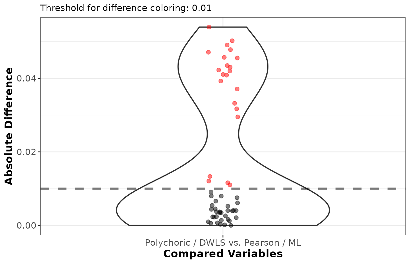
The two solutions agree on the structure, but the polychoric loadings are systematically a little larger: treating the items as continuous attenuates the loadings, because the Pearson correlation understates the latent associations. With only four categories here the gap is modest, but it widens as the number of categories drops (it is largest for binary items) and as the category thresholds grow more asymmetric (skewed items). This is why a polychoric or tetrachoric treatment is preferable for genuinely ordinal items with few categories.
The polychoric route does make its own demands, though: it assumes a normal latent variable underlies each item, and it needs an adequate sample size and reasonably populated response-category combinations. When categories are very sparse (rare responses, small samples), the polychoric asymptotic covariance behind the DWLS weights and the robust standard errors becomes unreliable, and collapsing rare categories can help.
Missing Data
When some responses are missing, dropping every incomplete case
(listwise deletion) wastes data and can bias the results unless the
values are missing completely at random. EFAtools offers
two principled alternatives that assume only that the data are missing
at random (MAR): a single-analysis route via full-information maximum
likelihood, and a multiple-imputation route via
efa_mi().
We simulate 250 continuous cases with about 15% of values missing at
random, where each item’s missingness depends on another item’s value.
By default, efa_simulate() would make each item’s
missingness depend on another item that is itself partly missing — a
kind of missingness the two routes below are not designed for. Rather
than failing outright, they run with a residual bias that grows as
missing_prop and missing_strength
increase.
missing_vars and missing_predictor avoid
that. Here the first nine items carry the missing values and each is
driven by one of the last nine, which stay complete. Every predictor is
therefore fully observed, satisfying the ignorable MAR
assumption the two routes below rely on – not just MAR, but MAR with no
incomplete predictor left unaccounted for.
d_miss <- efa_simulate(N = 250, Lambda = Lambda, Phi = Phi,
                       missing = "MAR", missing_prop = 0.15,
                       missing_vars = 1:9, missing_predictor = 10:18,
                       seed = 2024)$data
round(mean(is.na(d_miss)), 3)          # overall proportion missing
#> [1] 0.078
round(colMeans(is.na(d_miss)), 3)      # holed items only
#>    V1    V2    V3    V4    V5    V6    V7    V8    V9   V10   V11   V12   V13
#> 0.172 0.132 0.184 0.160 0.140 0.152 0.156 0.156 0.144 0.000 0.000 0.000 0.000
#>   V14   V15   V16   V17   V18
#> 0.000 0.000 0.000 0.000 0.000
Two-Stage Full-Information Maximum Likelihood
With cor_method = "fiml", efa_fit()
estimates the saturated mean and covariance from all the observed data
by an EM algorithm (assuming the data are MAR) and analyses the
resulting correlation — a single fit that uses every case rather than
only the complete ones. The model fit is reported as corrected two-stage
(Satorra-Bentler) statistics.
efa_fiml <- efa_fit(d_miss, n_factors = 3, cor_method = "fiml", estimator = "ml",
                    rotation = "oblimin")
efa_fiml
#>
#> EFA performed with estimator = 'ML' and rotation = 'oblimin'
#>   (two-stage FIML correlations, N = 250).
#>
#> ── Rotated Loadings ────────────────────────────────────────────────────────────
#>
#>        F1     F2     F3    h2    u2
#> V1   -.029   .554  -.029  .293  .707
#> V2    .069   .613  -.092  .402  .598
#> V3   -.008   .630  -.018  .391  .609
#> V4    .194   .515   .051  .388  .612
#> V5   -.044   .575   .013  .316  .684
#> V6   -.044   .647   .095  .423  .577
#> V7   -.034   .028   .578  .330  .670
#> V8   -.022   .006   .684  .462  .538
#> V9    .163   .022   .511  .335  .665
#> V10   .021   .001   .550  .309  .691
#> V11   .008  -.008   .589  .348  .652
#> V12  -.057  -.041   .577  .317  .683
#> V13   .590  -.061   .115  .371  .629
#> V14   .471   .185   .090  .351  .649
#> V15   .688  -.056  -.097  .427  .573
#> V16   .627  -.044   .003  .376  .624
#> V17   .677   .073  -.044  .485  .515
#> V18   .546   .072   .027  .340  .660
#>
#> Legend:
#>   bold = |loading| >= .300
#>   grey = below cutoff
#>   red h2/u2 = Heywood-relevant value
#>
#> ── Factor Intercorrelations ────────────────────────────────────────────────────
#>
#>       F1     F2     F3
#> F1  1.000
#> F2   .358  1.000
#> F3   .247   .129  1.000
#>
#> ── Variances Accounted for ─────────────────────────────────────────────────────
#>
#>                      F1     F2     F3
#> SS loadings        2.339  2.206  2.119
#> Prop Tot Var        .130   .123   .118
#> Cum Prop Tot Var    .130   .252   .370
#> Prop Comm Var       .351   .331   .318
#> Cum Prop Comm Var   .351   .682  1.000
#>
#> ── Model Fit ───────────────────────────────────────────────────────────────────
#>
#> scaled χ²(102) = 111.53, p = .244
#> CFI: .99
#> TLI: .99
#> RMSEA [90% CI]: .02 [.00; .04]
#> SRMR: .04
The solution again recovers the three factors, and the printout
records that the correlation was obtained by two-stage FIML. Standard
errors are available here too: for estimator = "ML" or
"ULS", se = "information" or
"sandwich" return the corrected two-stage standard errors,
and se = "np-boot" works with any estimator.
FIML estimates the model from every case, but it does not fill in the
missing values. Any step that needs complete rows is therefore still
complete-case. efa_scores(d_miss, f = efa_fiml), for
example, scores only the complete cases and warns that the rest are
NA:
sum(complete.cases(d_miss))    # cases a score can be formed for
#> [1] 63
Use the efa_mi() route below if you want case-level
scores for every respondent. Each imputed dataset is complete, so
scoring it with the pooled loadings covers all 250 cases.
The correction itself needs a well-behaved saturated covariance. When
that cannot be formed — typically in a small sample with a high
proportion of missing values, or with near-collinear items —
efa_fit() warns and keeps the plain two-stage
likelihood-ratio statistic instead of discarding the test. Such a fit is
never presented as corrected: the printed chi-square line is labelled
uncorrected, and the accompanying p-value,
CFI, TLI, and RMSEA should be read as indicative only.
Multiple Imputation with efa_mi()
The alternative is to impute the missing values several times, fit
each completed dataset, and pool the results. EFAtools does
not impute the data itself — use a dedicated tool such as the mice package — but
efa_mi() takes the list of completed datasets and does the
factor-analytic pooling.
Here we create five imputations with mice (a Bayesian linear-regression model, appropriate for these continuous items) and collect them into a list.
imp <- mice::mice(as.data.frame(d_miss), m = 5, method = "norm",
                  printFlag = FALSE, seed = 123)
dat_list <- lapply(seq_len(imp$m), function(i) mice::complete(imp, i))
efa_mi() fits the same efa_fit() model to
each imputed dataset — the extraction, rotation, and standard-error
options are passed through ... — aligns the solutions to a
common factor space (rotation is only identified up to reflection and
permutation, so the imputations must be matched before averaging), and
pools them.
efa_pooled <- efa_mi(dat_list, n_factors = 3, estimator = "ml", rotation = "oblimin")
efa_pooled
#>
#> Pooled EFA across 5 imputations performed with estimator = 'ML' and
#>   rotation = 'oblimin' (N = 250).
#> Pooling settings: target_method = 'first_target',
#>   align_unrotated = 'signed_tucker_congruence', fit_pool_method = 'D2'.
#>
#> ── Rotated Loadings ────────────────────────────────────────────────────────────
#>
#>        F1     F2     F3    h2    u2
#> V1   -.018   .573  -.013  .320  .680
#> V2    .058   .605  -.082  .385  .615
#> V3    .019   .604  -.019  .370  .630
#> V4    .209   .494  -.005  .359  .641
#> V5   -.076   .610   .002  .346  .654
#> V6   -.044   .640   .095  .415  .585
#> V7   -.011  -.003   .550  .299  .701
#> V8   -.013   .022   .654  .428  .572
#> V9    .162   .045   .512  .340  .660
#> V10   .027  -.002   .553  .313  .687
#> V11   .018  -.011   .577  .336  .664
#> V12  -.054  -.042   .581  .323  .677
#> V13   .587  -.054   .116  .368  .632
#> V14   .471   .181   .097  .349  .651
#> V15   .692  -.071  -.086  .431  .569
#> V16   .630  -.051   .007  .379  .621
#> V17   .668   .079  -.031  .480  .520
#> V18   .545   .082   .040  .347  .653
#>
#> Legend:
#>   bold = |loading| >= .300
#>   grey = below cutoff
#>   red h2/u2 = Heywood-relevant value
#>
#> ── Factor Intercorrelations ────────────────────────────────────────────────────
#>
#>       F1     F2     F3
#> F1  1.000
#> F2   .349  1.000
#> F3   .227   .136  1.000
#>
#> ── Variances Accounted for ─────────────────────────────────────────────────────
#>
#>                      F1     F2     F3
#> SS loadings        2.347  2.197  2.044
#> Prop Tot Var        .130   .122   .114
#> Cum Prop Tot Var    .130   .252   .366
#> Prop Comm Var       .356   .333   .310
#> Cum Prop Comm Var   .356   .690  1.000
#>
#> ── Model Fit ───────────────────────────────────────────────────────────────────
#>
#> D2-pooled χ²(102) = 111.01, p = .488
#> CFI (avg. over imputations): .93
#> TLI (avg. over imputations): .90
#> RMSEA [90% CI]: .02 [.00; .04]
#> SRMR: .04
#> Note: the pooled χ² is the D2 statistic; its p uses the D2 reference F(102,
#> 9.0), not the χ²(102) tail.
#> Note: CFI and TLI are averaged over the imputations, not formed from the
#> separately pooled model and baseline statistics in `mi_diagnostics`.
The pooled loadings recover the three factors. Point estimates are
averaged across the imputations after alignment. The model chi-square,
and the AIC/BIC derived from it, are pooled with the same rule as RMSEA,
but applied to a different discrepancy scale — which is why the printout
labels the pooled chi-square D2-pooled, and why you
should not expect it to reconcile by hand with the pooled RMSEA. The
incremental CFI and TLI are instead averaged across the per-imputation
fits. Requesting standard errors in the call (for example
se = "information" or se = "np-boot")
additionally pools them with Rubin’s rules, so the between-imputation
variability inflates the pooled standard errors. Because multiple
imputation propagates the extra uncertainty from the missing data, its
pooled fit statistics are not directly comparable with the single FIML
fit above; read them together with the per-imputation fits stored in the
returned object.
Which route to prefer is largely practical. FIML is a single, efficient fit and is the simpler default when the analysis model is the whole story. Multiple imputation is more flexible when the imputation model should draw on auxiliary variables not in the factor model, or when the same imputations feed several downstream analyses.
Ordinal and Missing Data
Questionnaire data are usually both: a few response categories and some unanswered items. The two treatments above do not simply combine, because the ordinal machinery needs complete cases exactly where the FIML route needs continuous ones. We draw the same four-category items as before, now with 8% of the responses missing completely at random.
d_ord_miss <- efa_simulate(N = 300, Lambda = Lambda, Phi = Phi,
                           categories = 4, match = "polychoric",
                           missing = "MCAR", missing_prop = 0.08, seed = 2024)$data

round(mean(is.na(d_ord_miss)), 3)     # overall proportion missing
#> [1] 0.083
sum(complete.cases(d_ord_miss))       # respondents who answered every item
#> [1] 62
Eight percent per item is mild, but spread over 18 items it leaves only a fifth of the sample complete. That number, not the 300 rows supplied, is what the ordinal route has to work with.
The Effective Sample of a Polychoric DWLS Fit
Polychoric correlations can be estimated pair by pair, using every
respondent who answered a given pair of items. Their asymptotic
covariance cannot: the DWLS weights and the sandwich standard errors
describe one set of estimates from one set of cases,
so whenever they are requested the correlations and the covariance are
both computed on the listwise-complete rows. efa_fit()
announces that override rather than applying it silently.
efa_ord_miss <- efa_fit(d_ord_miss, n_factors = 3, cor_method = "poly",
                        estimator = "dwls", rotation = "oblimin")
#> ℹ An asymptotic covariance requires complete cases, so 238 of 300 rows with
#>   missing values were dropped (listwise; N = 62). This overrides `use =
#>   "pairwise.complete.obs"`.
efa_ord_miss$settings$N        # cases the fit is actually based on
#> [1] 62
Every loading, fit index, standard error, and confidence interval of
that fit rests on the complete cases. efa_screen() names
both denominators for the same reason — its multivariate-normality and
outlier results state how many complete cases they used out of how many
rows were supplied — so the reduction is visible before a model is
fitted.
Two adjustments avoid it, each with a cost:
- Ask for no asymptotic covariance. With
estimator = "ULS"or"ML"and no sandwich standard errors, nothing needs the weight matrix, so the polychoric matrix stays pairwise-complete and every case contributes to the pairs it answered. In exchange you give up the DWLS weighting and the robust standard errors, and the reportedNis the nominal row count while each correlation rests on its own smaller subset — so fit statistics and analytic standard errors treat the data as more complete than they are, andefa_fit()warns about this. - Switch to FIML — but only as a continuous analysis.
cor_method = "fiml"estimates a saturated normal covariance and analyses the resulting Pearson-type correlation; there is no polychoric asymptotic covariance in it, so it cannot supply DWLS with weights. Combining the two is refused rather than silently approximated:
efa_fit(d_ord_miss, n_factors = 3, cor_method = "fiml", estimator = "dwls")
#> Error in `efa_fit()`:
#> ! `estimator = "DWLS"` cannot be used with `cor_method = "fiml"`.
#> ℹ DWLS needs polychoric correlations. With FIML, use "ML", "ULS", or "PAF".
Keeping Both the Ordinal Treatment and the Cases
Multiple imputation is the route that keeps both. Each imputed
dataset is complete, so the polychoric correlations and their asymptotic
covariance are estimated on all 300 cases, and the imputation
uncertainty is carried into the pooled results. Since
efa_mi() forwards its arguments to efa_fit(),
this is the ordinal fit above applied to each imputation — here with
predictive mean matching, which resamples observed values and so
respects the response scale.
imp_ord <- mice::mice(as.data.frame(d_ord_miss), m = 5, method = "pmm",
                      printFlag = FALSE, seed = 123)
dat_ord <- lapply(seq_len(imp_ord$m), function(i) mice::complete(imp_ord, i))

efa_ord_pooled <- efa_mi(dat_ord, n_factors = 3, cor_method = "poly",
                         estimator = "dwls", rotation = "oblimin")
efa_ord_pooled
#>
#> Pooled EFA across 5 imputations performed with estimator = 'DWLS' and
#>   rotation = 'oblimin' (polychoric correlations, N = 300).
#> Pooling settings: target_method = 'first_target',
#>   align_unrotated = 'signed_tucker_congruence', fit_pool_method = 'D2'.
#>
#> ── Rotated Loadings ────────────────────────────────────────────────────────────
#>
#>        F1     F2     F3    h2    u2
#> V1   -.060   .538   .092  .317  .683
#> V2   -.059   .544  -.021  .285  .715
#> V3    .033   .581   .020  .352  .648
#> V4    .049   .583   .091  .392  .608
#> V5    .088   .700  -.111  .474  .526
#> V6   -.014   .573  -.005  .325  .675
#> V7    .049   .082   .533  .339  .661
#> V8    .010  -.016   .618  .381  .619
#> V9    .135   .038   .473  .304  .696
#> V10   .012  -.042   .726  .517  .483
#> V11  -.035   .019   .577  .325  .675
#> V12  -.024  -.004   .585  .331  .669
#> V13   .647  -.017   .019  .425  .575
#> V14   .717   .052  -.088  .484  .516
#> V15   .614   .056   .081  .437  .563
#> V16   .520  -.118  -.012  .264  .736
#> V17   .544   .022   .050  .323  .677
#> V18   .570   .057   .020  .347  .653
#>
#> Legend:
#>   bold = |loading| >= .300
#>   grey = below cutoff
#>   red h2/u2 = Heywood-relevant value
#>
#> ── Factor Intercorrelations ────────────────────────────────────────────────────
#>
#>       F1     F2     F3
#> F1  1.000
#> F2   .137  1.000
#> F3   .381   .289  1.000
#>
#> ── Variances Accounted for ─────────────────────────────────────────────────────
#>
#>                      F1     F2     F3
#> SS loadings        2.288  2.144  2.191
#> Prop Tot Var        .127   .119   .122
#> Cum Prop Tot Var    .127   .246   .368
#> Prop Comm Var       .346   .324   .331
#> Cum Prop Comm Var   .346   .669  1.000
#>
#> ── Model Fit ───────────────────────────────────────────────────────────────────
#>
#> SRMR: .04
#> df: 102
#>
#> Note: With `estimator = "DWLS"`, the chi-square test and the fit indices
#> derived from it (CFI, TLI, RMSEA, AIC, BIC, ECVI) are not available; refit with
#> `se = "sandwich"` for the scaled chi-square.
The pooled pattern matrix is estimated from all 300 respondents
rather than the 62 complete ones — compare it with
efa_ord_miss$rot_loadings — and the between-imputation
variability enters any pooled standard errors requested in the call. As
always with imputation, the imputation model has to be defensible: for
ordinal items that means a method returning values on the observed scale
(predictive mean matching, or an ordinal model such as
method = "polr"), and enough respondents per item to
estimate it.
So, for ordinal items with missing values: use efa_mi()
when the missingness is more than incidental and the ordinal treatment
matters; fit cor_method = "poly" with
estimator = "DWLS" directly when the complete-case sample
is still comfortably large; and use FIML when the items have enough
categories to be treated as continuous in the first place.
Where to Next
This vignette covered the ordinal and missing-data extensions of the
workflow. For the core analysis — screening, factor retention,
extraction and rotation, and the post-processing tools — see the EFAtools vignette, and the individual help
pages for the statistical details and references. Run
browseVignettes("EFAtools") for the vignettes installed
with the package, or visit the package website for the
full set of articles.