Confirmatory Factor Analysis

Markus Steiner

Institute for Mental and Organisational Health, FHNW

06 June, 2025

CFA

Each indicator is allocated to a factor, other loadings fixed to 0 \(\rightarrow\) achieves simple structure; no rotation necessary.
Loadings can be fixed to specific values or constrained to equality.
Uniquenesses can be correlated (e.g. to account for wording effects).
More parsimonious than EFA due to fixed parameters.

When to use CFA

Scale construction
- Reliability
- Construct validity (discriminant and convergent)
- Method bias (MTMM)
- Scoring
- Test for a general factor
Testing measurement models in SEM
Model measurement error
Test measurement invariance

Specifying a Factor Model – Path Diagram

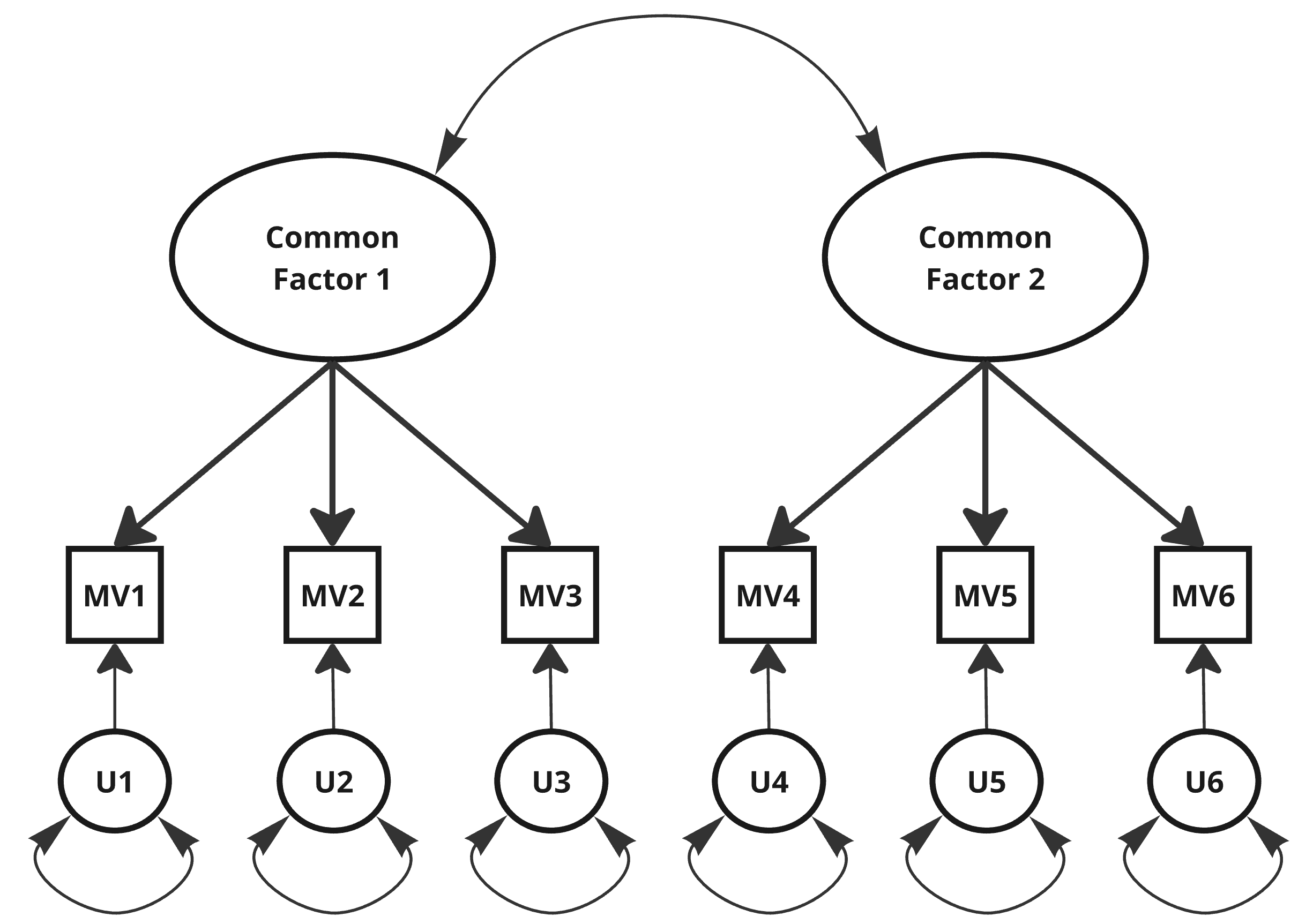
Specifying a Factor Model – `{lavaan}`

{lavaan}-Syntax:
- =~ denotes a latent variable measured by indicators.
- By default, covariances between CFs are free.
Fit the model with lavaan::cfa() (you can also use lavaan::sem()).
Obtain Output with summary()

model <- '
  CF1 =~ MV1 + MV2 + MV3
  CF2 =~ MV4 + MV5 + MV6
'
fit <- lavaan::cfa(model, data = your_data)
summary(fit, fit.measures = TRUE, standardized = TRUE)

Scaling the Latent Variable

A latent variable is unobserved and must have its scale identified.
Usually, one of two ways:
- Marker or reference indicator.
  - Most popular method and default in {lavaan} (first MV per CF).
  - Provides an unstandardized solution.
- Fixing the variance to a specific value, usually 1.
  - Provides a partially standardized solution.

Model Identification - I

Based on difference between information in input matrix and freely estimated parameters.
Three possibilities:
- Underidentified model \(\rightarrow\) More unknown than known values (negative \(df\)s).
- Just-identified model \(\rightarrow\) Equal number of unknown and known values (0 \(df\)s).
- Overidentified model \(\rightarrow\) Fewer unknown than known values (positive \(df\)s).
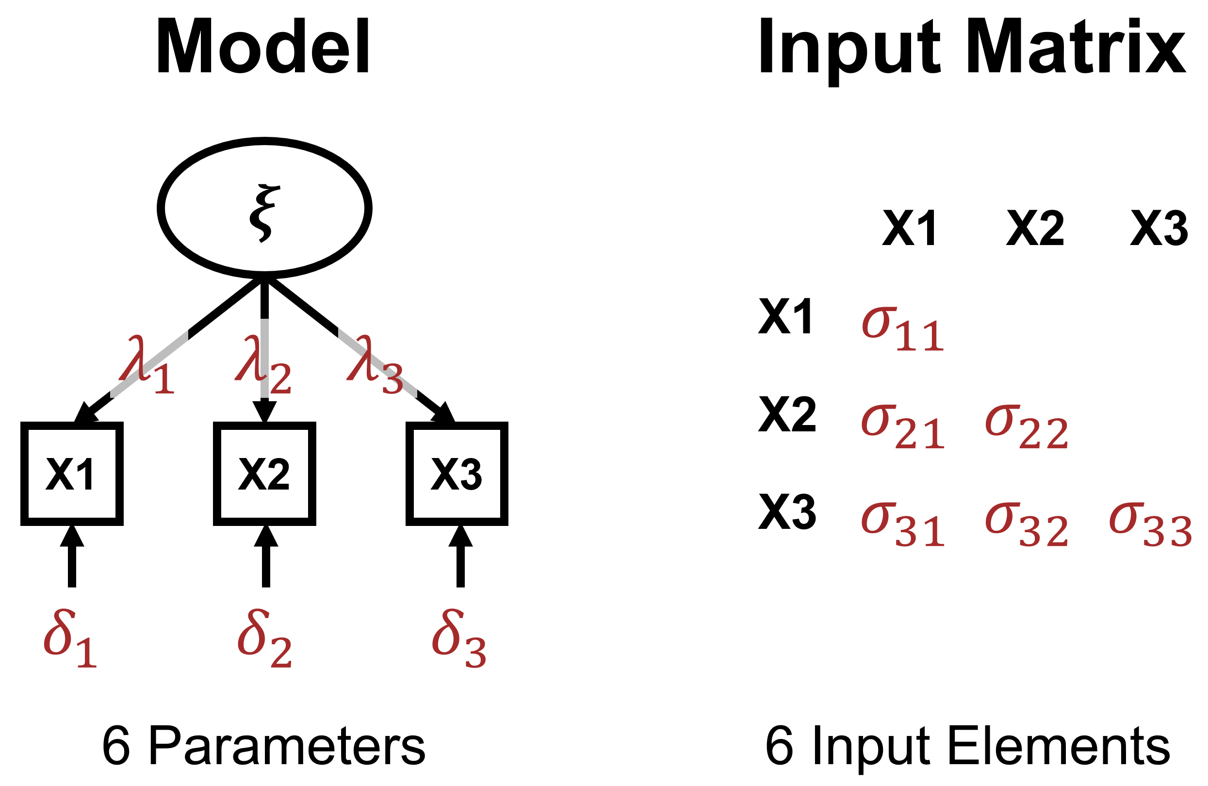
Number of input elements with \(p\) MVs: \(p(p+1)/2\)

Underidentification

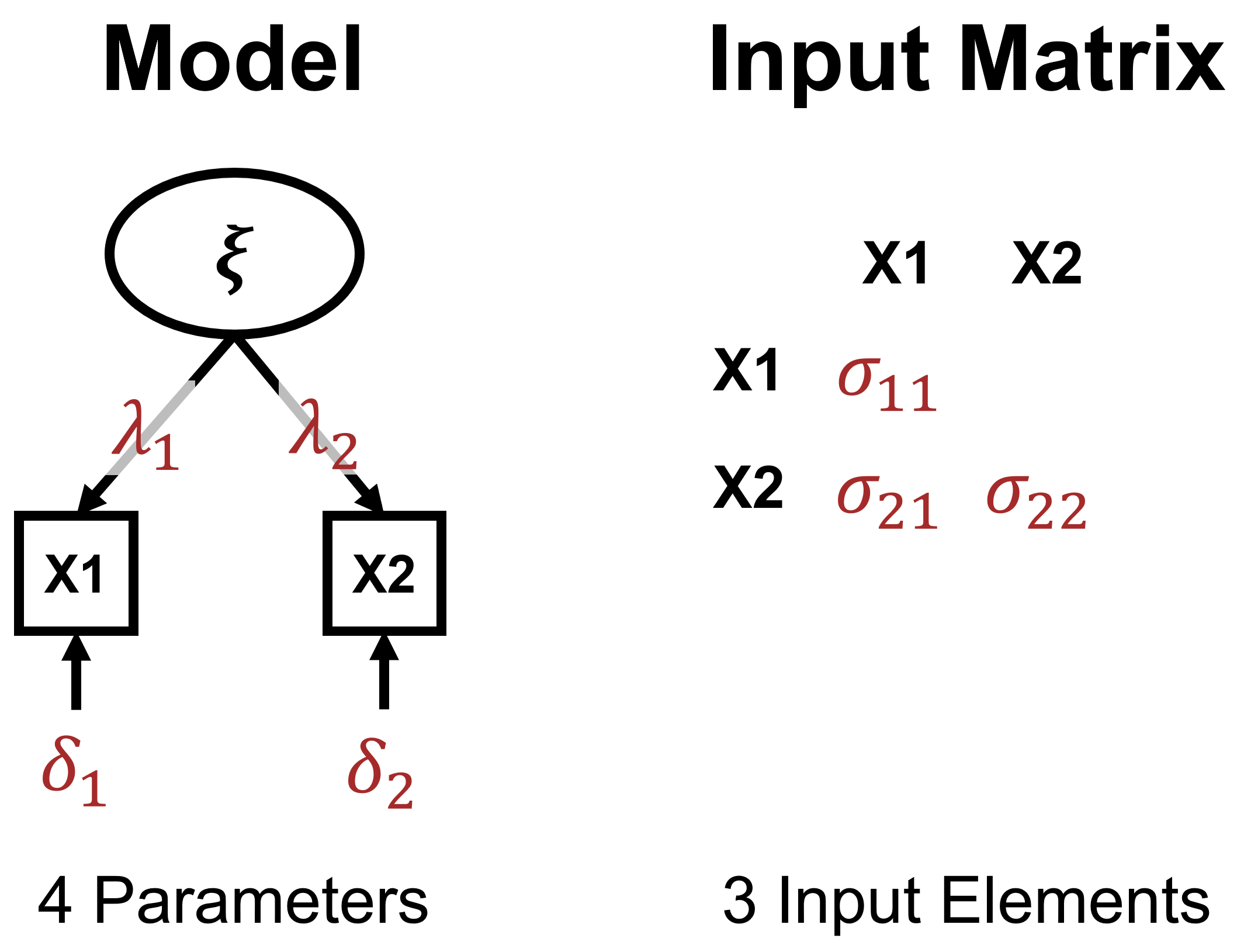
Just-Identification

Overidentification

Model Identification - II

CFs must be scaled
# input elements \(\geq\) # freely estimated model parameters
Overidentification with two or more MVs per CF from two factors on, but min three MVs per CF should be used to avoid empirical underidentification

Model Estimation

When using maximum likelihood (ML) estimation, parameters are found by minimizing

\[F_{ML}=ln|S| - ln|\Sigma| + trace(S\Sigma^{-1})-p\]

\(S\): Sample covariance matrix
\(\Sigma\): Model-implied covariance matrix
p: Number of indicators

\(\rightarrow\) Perfect fitting model, \(S\) and \(\Sigma\) are identical, so \(F_{ML}\) is 0, as \(S\Sigma^{-1}=I\) and thus \(trace(S\Sigma^{-1})=p\).

Model Fit - \(\chi^2\)

\(F_{ML}(N-1)\) is approx. \(\chi^2\)-distributed.
\(\rightarrow\) Significance test, whether discrepancy between \(S\) and \(\Sigma\) is negligible.
Problems:
- Unreasonable premise
- Needs large enough sample and normal data
- Inflated with very large samples, i.e., oversensitive.
- \(\rightarrow\) Therefore, additional fit indices are considered

Model Fit - Indices

Absolute fit indices, e.g.:

RMSEA (\(\leq\).05, Hu & Bentler, 1999; but dependent on \(N\), \(df\), and model-specification F. Chen et al., 2008; Kenny et al., 2015)
SRMR/CRMR (SRMR \(\leq\).08, Hu & Bentler, 1999)

Incremental fit indices, e.g. (reduction in misfit compared to baseline, usually zero covariances):

TLI (\(\geq\).95, Hu & Bentler, 1999)
CFI (\(\geq\).95, Hu & Bentler, 1999)

\(\rightarrow\) Report multiple indices (F. Chen et al., 2008; Hu & Bentler, 1999; Moshagen & Auerswald, 2018).

\(\rightarrow\) Don’t overrely on cut-off values (F. Chen et al., 2008; Kenny et al., 2015; Lai & Green, 2016).

\(\rightarrow\) RMSEA and TLI good measures of fit and fitting propensity according to (Bader & Moshagen, 2025), but see also (Bonifay et al., 2025).

Cut-offs…

Practical exoperience has made us feel that a value of the RMSEA of about 0.05 or less would indicate a close fit of the model in relation to the degrees of freedom.

Browne & Cudeck (1993), p.144

In our experience, models with overall fit indices of less than .90 can usually be improved substantially.

Bentler & Bonett (1980), p. 600

\(\rightarrow\) But many simulation studies since (see previous slide).

Model Evaluation

Global/overall fit
Local fit
Interpretability, size, and stat. significance of model parameters

Model Evaluation - Global Fit

Is the \(\chi^2\)-test significant?
Are the fit indices within the acceptable range?
\(\rightarrow\) Can provide conclusive evidence for misfit, but not for good fit of the model.

Model Evaluation - Local Fit I

Standardized Residual variances:
- \(S-\Sigma\) divided by SEs.
- Interpretable as z-Scores, i.e., absolute values of 2 or 2.58 (for large samples) indicate significant differences on 5% and 1% \(\alpha\)-level.
- Positive values: Model underestimates relationship.
- Negative values: Model overestimates relationship.
- Transform \(S\) and \(\Sigma\) to correlation matrices, then \(\Delta > .1\)? (Kline, 2023)
Modification Indices (MI): Approx. of decrease in \(\chi^2\) if a spec. parameter is freed.
- Substantial improvement if \(\geq 3.84\) (crit. value of \(\chi^2\) distribution with 1 \(df\))
- Substantive reasons should exist for relaxing constraints.
- Freeing one parameter can affect multiple MIs.
- Problem of overfitting.

Model Evaluation - Local Fit II

Expected Parameter Change (EPC):
- How large is the change in a parameter if it is freed.
- Given together with MIs.
Univariate Wald Test:
- Opposite of MI: is model sign. worse if a parameter is fixed to 0.
- If \(< 3.84\).
- This is how the sign. of the parameters are calculated.
Further ressource on local fit, esp. in the SEM case: Thoemmes et al. (2018)

Model Evaluation - Model Parameters

Are parameters substantial (i.e., sign. different from 0)?
No Heywood cases should be present.
Non-positive-definite matrix indicates problems.
Estimates should make sense (i.e., sign and size of loadings and correlations).
Size/variability of standard errors (problems can stem from misspecified model, non-normal data, small N, or other issues).
Communalities should be substantial.

Interpretation of Parameters

Unstandardized solution:
- Parameter estimates are based on the original metrics of the indicators and factors.
- Factor loadings are unstandardized regression coefficients.
Partially standardized solution:
- Indicators are unstandardized and latent variables are standardized or vice versa.
Completely standardized solution:
- Metrics of both indicators and latent variables are standardized (M = 0, SD = 1).
- Loadings are standardized regression coefficients (between -1 and 1).

Model Evaluation in `{lavaan}`

Fit the model with cfa()
Obtain model fit and parameters with summary()
Look at (standardized) residuals with lavResiduals()
Inspect MIs and EPCs with modindices()

model <- '
  CF1 =~ MV1 + MV2 + MV3
  CF2 =~ MV4 + MV5 + MV6
'
fit <- lavaan::cfa(model, data = your_data)
summary(fit, fit.measures = TRUE, standardized = TRUE)
lavResiduals(fit)
modindices(fit, sort = TRUE)

Exercises

Sections A and B in the CFA exercises

Revising the Model

To improve fit if global/local fit problems or problems in parameters
- Based on MIs/EPCs and substantive reasons \(\rightarrow\) free MIs one-by-one: do the other MIs vanish or stay?
- Note: MIs cannot tell whether to add correlated residuals or add a factor.
To improve parsimony and interpretability
- Collapsing highly correlated factors
- Higher-order models

More {lavaan} syntax:

# add a cross-loading
model <- '
  CF1 =~ MV1 + MV2 + MV3
  CF2 =~ MV4 + MV5 + MV6 + MV2
'

# add a cov between residuals of MV3 and MV6
model <- '
  CF1 =~ MV1 + MV2 + MV3
  CF2 =~ MV4 + MV5 + MV6
  MV3 ~~ MV6
'

# constrain or fix parameters
model <- '
  CF1 =~ a*MV1 + a*MV2 + a*MV3
  CF2 =~ MV4 + MV5 + MV6
  CF1 ~~ 0*CF2
'

Model comparison

Nested models: \(\chi^2\)-test or information criteria
Non-nested models: Information criteria and general fit

# LRT
lavTestLRT(model_1, model_2)

Visualizing the Model

Two approaches:

Use R package
- {semPlot}
- {lavaanPlot}
Do it by hand
- Power Point/ Keynote
- draw.io
- …

# using {semPlot}
semPaths(lavaan_model, 'std', 'std', style = "lisrel")

# using {lavaanPlot}
lavaanPlot(lavaan_model, coefs = TRUE, stand = TRUE, covs = TRUE)

Exercises

Sections C to E in the CFA exercises

“Special” Data

Non-normal: Robust ML with non-normal continuous data
Categorical: DWLS with polychoric correlations
- Note: Fit indices may be biased or not interpretable as usual (e.g., Savalei, 2021; Shi & Maydeu-Olivares, 2020; Xia & Yang, 2019) \(\rightarrow\) focus on the Scaled statistics in the {lavaan} output.
Small datasets: Use bounded estimation to avoid convergence issues (see, De Jonckere & Rosseel, 2022)

model <- '
  CF1 =~ MV1 + MV2 + MV3
  CF2 =~ MV4 + MV5 + MV6
'
# non-normal data:
# robust standard errors and scaled test statistic
fit <- lavaan::cfa(model, data = your_data,
                   se = "robust", test = "Satorra-Bentler")
# categorical data 
fit <- lavaan::cfa(model, data = your_data,
                   ordered = TRUE)

# small datasets
fit <- lavaan::cfa(model, data = your_data,
                   bounds = "standard")
summary(fit, fit.measures = TRUE, standardized = TRUE)

Missing Data

Pairwise and listwise deletion: Not efficient and potentially biased
Simple/single imputation: Underestimates variances and SEs and overestimates correlations
Instead use:
- Direct ML / FIML: Needs multivariate normal distribution
- Multiple imputation: Random noise is added to regression prediction (needs {mice} and {lavaan.mi})

model <- '
  CF1 =~ MV1 + MV2 + MV3
  CF2 =~ MV4 + MV5 + MV6
'

# FIML
fit <- lavaan::cfa(model, data = your_data,
                   missing = "ml") # or "fiml" or "direct"

# Multiple imputation with {mice} (simplified)
data_imp <- mice(data = your_data %>% 
                   mutate(across(MV1:MV6, ordered)),
                 method = "polr")
data_imp <- map(seq_len(5),
                ~complete(data_imp, action = .x, inc = FALSE))

# fit with {lavaan.mi}
fit_imp <- cfa.mi(model, data = data_imp, ordered = TRUE)

Exercises

Sections F and G in the CFA exercises

Measurement invariance

Compare solutions between groups (e.g., gender, language, etc.)
Levels:
- Configural invariance: Equality of number of factors and pattern of indicator-factor loadings
- Metric invariance / weak factorial invariance: Equality of factor loadings
- Scalar invariance / strong factorial invariance: Equality of indicator intercepts
- Strict factorial invariance: Equality of indicator residuals
Sequential tests using \(\chi2\)-tests and GOF-measures of constrained and unconstrained models.
\(\Delta\) Fit indices: see F. F. Chen (2007):
- Loadings invariant if: \(\Delta CFI \leq -.005\) and \(\Delta RMSEA \geq .010\) or \(\Delta SRMR \geq .025\)
- Intercept or residuals invariant if: \(\Delta CFI \leq -.005\) and \(\Delta RMSEA \geq .010\) or \(\Delta SRMR \geq .005\)
Partial measurement invariance: Only some parameters invariant \(\rightarrow\) free others.

Measurement invariance in `{lavaan}`

Fit different models with cfa() and arguments group and group.equal specified.
Compare using lavTestLRT()
Compare fit measures (fitMeasures())
(semTools::measEq.syntax() can help generating model syntax)

model <- '
  CF1 =~ MV1 + MV2 + MV3
  CF2 =~ MV4 + MV5 + MV6
'

# configural invariance
fit_conf <- cfa(model, data = your_data, group = "group_var")

# weak invariance
fit_weak <- cfa(model, data = your_data, group = "group_var",
                group.equal = "loadings")

# strong invariance
fit_strong <- cfa(model, data = your_data, group = "group_var",
                  group.equal = c("intercepts", "loadings"))

# model comparison tests
lavTestLRT(fit_conf, gad7_2f_wfit_weakeak, fit_strong)

# obtain fit measures of interest
fitMeasures(fit_conf)[c("cfi", "rmsea", "srmr")]

Exercises

Section H in the CFA exercises

Higher-Order Models

Capture covariation among factors with a higher order factor \(\rightarrow\) factor correlations are input for second-order factor analysis
Sequence:
- Fit a first-order CFA solution that fits well
- Examine magnitude and pattern for factor intercorrelations
- Fit second-order factor model, as justified on conceptual and empirical grounds

model <- '
  CF1 =~ MV1 + MV2 + MV3
  CF2 =~ MV4 + MV5 + MV6
  CF3 =~ MV7 + MV8 + MV9
  CF4 =~ MV10 + MV11 + MV12
  
  # higher-order factor
  HOF =~ CF1 + CF2 + CF3 + CF4
'

fit <- lavaan::cfa(model, data = your_data)
summary(fit, fit.measures = TRUE, standardized = TRUE)

Exercises

Section I in the CFA exercises

Reporting a CFA (Brown, 2015, p. 129) - I

Model specification:

Justification for hypothesized model
Complete description of parameter specifications:
- List indicators per factor.
- How were the CFs scaled (e.g., which MVs were used as indicator variables).
- Describe free, fixed, and constrained parameters.
Demonstrate that model is identified (e.g., positive \(df\)).

Reporting a CFA (Brown, 2015, p. 129) - II

Input data:

Sample characteristics, sample size, sampling method.
Type of data used (e.g., nominal, ordina, interval; scale range of indicators).
Tests of estimator assumptions (e.g., multivariate normality).
Missing data and handling thereof (e.g., FIML, multiple imputation).
Provide sample correlation matrix and indicator SDs (and means if applicable).

Reporting a CFA (Brown, 2015, p. 129) - III

Model estimation:

Software and version.
Type of data analyzed (e.g., variance-covariance; polychorric correlations)
Estimator used (e.g., ML, WLS), as justified by properties of data.

Reporting a CFA (Brown, 2015, p. 129) - IV

Model evaluation:

Global fit
- \(\chi^2\) with \(df\) and \(p\)
- Multiple fit indices (e.g., RMSEA, TLI), incl. CIs, if appl., and cut-offs used.
Local fit
- Strategies used for local fit assessment.
- Absence of areas of ill fit or indicate areas of strain in model.
If model is respecified, provide compelling substantive rationale and document improvement in fit.
Parameter estimates
- Report all estimates, including nonsign. ones.
- Consider practical and statistical sign. of estimates.
- Include SEs or CIs of parameters.
If necessary, report steps to verify power and precision of model.

Reporting a CFA (Brown, 2015, p. 129) - V

Substantive conclusions:

Discuss CFA results regarding their implications.
Interpret findings in context of study limitations and other considerations (e.g., equivalent models).

Exercises

Sections J in the CFA exercises

References

Bader, M., & Moshagen, M. (2025). Assessing the fitting propensity of factor models. Psychological Methods, 30(2), 254–270. https://doi.org/10.1037/met0000529

Bentler, P. M., & Bonett, D. G. (1980). Significance tests and goodness of fit in the analysis of covariance structures. Psychological Bulletin, 88(3), 588–606. https://doi.org/10.1037/0033-2909.88.3.588

Bonifay, W., Cai, L., Falk, C. F., & Preacher, K. J. (2025). Reassessing the fitting propensity of factor models. Psychological Methods. https://doi.org/10.1037/met0000735

Brown, T. A. (2015). Confirmatory Factor Analysis for Applied Research (2nd ed.). The Guilford Press.

Browne, M. W., & Cudeck, R. (1993). Alternative ways of assessing model fit. In K. A. Bollen & J. S. Long (Eds.), Testing structural equation models (pp. 136–162). Sage.

Chen, F. F. (2007). Sensitivity of Goodness of Fit Indexes to Lack of Measurement Invariance. Structural Equation Modeling: A Multidisciplinary Journal, 14(3), 464–504. https://doi.org/10.1080/10705510701301834

Chen, F., Curran, P. J., Bollen, K. A., Kirby, J., & Paxton, P. (2008). An Empirical Evaluation of the Use of Fixed Cutoff Points in RMSEA Test Statistic in Structural Equation Models. Sociological Methods & Research, 36(4), 462–494. https://doi.org/10.1177/0049124108314720

De Jonckere, J., & Rosseel, Y. (2022). Using Bounded Estimation to Avoid Nonconvergence in Small Sample Structural Equation Modeling. Structural Equation Modeling: A Multidisciplinary Journal, 29(3), 412–427. https://doi.org/10.1080/10705511.2021.1982716

Hu, L., & Bentler, P. M. (1999). Cutoff criteria for fit indexes in covariance structure analysis: Conventional criteria versus new alternatives. Structural Equation Modeling: A Multidisciplinary Journal, 6(1), 1–55. https://doi.org/10.1080/10705519909540118

Kenny, D. A., Kaniskan, B., & McCoach, D. B. (2015). The Performance of RMSEA in Models With Small Degrees of Freedom. Sociological Methods & Research, 44(3), 486–507. https://doi.org/10.1177/0049124114543236

Kline, R. B. (2023). Principles and practice of structural equation modeling (5th ed.). The Guilford Press.

Lai, K., & Green, S. B. (2016). The Problem with Having Two Watches: Assessment of Fit When RMSEA and CFI Disagree. Multivariate Behavioral Research, 51(2-3), 220–239. https://doi.org/10.1080/00273171.2015.1134306

Moshagen, M., & Auerswald, M. (2018). On congruence and incongruence of measures of fit in structural equation modeling. Psychological Methods, 23(2), 318–336. https://doi.org/10.1037/met0000122

Savalei, V. (2021). Improving Fit Indices in Structural Equation Modeling with Categorical Data. Multivariate Behavioral Research, 56(3), 390–407. https://doi.org/10.1080/00273171.2020.1717922

Shi, D., & Maydeu-Olivares, A. (2020). The Effect of Estimation Methods on SEM Fit Indices. Educational and Psychological Measurement, 80(3), 421–445. https://doi.org/10.1177/0013164419885164

Thoemmes, F., Rosseel, Y., & Textor, J. (2018). Local fit evaluation of structural equation models using graphical criteria. Psychological Methods, 23(1), 27–41. https://doi.org/10.1037/met0000147

Xia, Y., & Yang, Y. (2019). RMSEA, CFI, and TLI in structural equation modeling with ordered categorical data: The story they tell depends on the estimation methods. Behavior Research Methods, 51(1), 409–428. https://doi.org/10.3758/s13428-018-1055-2

Confirmatory Factor Analysis

CFA

When to use CFA

Specifying a Factor Model – Path Diagram

Specifying a Factor Model – {lavaan}

Scaling the Latent Variable

Model Identification - I

Underidentification

Just-Identification

Overidentification

Model Identification - II

Model Estimation

Model Fit - \(\chi^2\)

Model Fit - Indices

Cut-offs…

Model Evaluation

Model Evaluation - Global Fit

Model Evaluation - Local Fit I

Model Evaluation - Local Fit II

Model Evaluation - Model Parameters

Interpretation of Parameters

Model Evaluation in {lavaan}

Exercises

Revising the Model

Model comparison

Visualizing the Model

Exercises

“Special” Data

Missing Data

Exercises

Measurement invariance

Measurement invariance in {lavaan}

Exercises

Higher-Order Models

Exercises

Reporting a CFA (Brown, 2015, p. 129) - I

Reporting a CFA (Brown, 2015, p. 129) - II

Reporting a CFA (Brown, 2015, p. 129) - III

Reporting a CFA (Brown, 2015, p. 129) - IV

Reporting a CFA (Brown, 2015, p. 129) - V

Exercises

References

Specifying a Factor Model – `{lavaan}`

Model Evaluation in `{lavaan}`

Measurement invariance in `{lavaan}`