CFA Exercises

Workshop: Introduction to Factor Analysis - GSP 2025

Author
Affiliation

Markus Steiner

Institute for Mental and Organisational Health, FHNW

Published

06 June, 2025

A – Setup

Exercise A1. Open the Intro2FactorAnalysis RStudio-Project and create a new R-script CFA_exercises.R.

Exercise A2. Load the following R-packages: lavaan, semTools, lavaan.mi, mice, semPlot, lavaanPlot and tidyverse.

Show Solution

library(lavaan)
This is lavaan 0.6-19
lavaan is FREE software! Please report any bugs.
library(semTools)
 
###############################################################################
This is semTools 0.5-7
All users of R (or SEM) are invited to submit functions or ideas for functions.
###############################################################################
library(lavaan.mi)
 
###################################################################
This is lavaan.mi 0.1-0
See the README file on github.com/TDJorgensen/lavaan.mi
for a table comparing it with deprecated semTools features.
###################################################################

Attache Paket: 'lavaan.mi'
Die folgenden Objekte sind maskiert von 'package:semTools':

    calculate.D2, cfa.mi, growth.mi, lavaan.mi, lavTestLRT.mi,
    lavTestScore.mi, lavTestWald.mi, modificationindices.mi,
    modificationIndices.mi, modindices.mi, sem.mi
library(mice)

Attache Paket: 'mice'
Das folgende Objekt ist maskiert 'package:stats':

    filter
Die folgenden Objekte sind maskiert von 'package:base':

    cbind, rbind
library(semPlot)
library(lavaanPlot)
library(tidyverse)
── Attaching core tidyverse packages ──────────────────────── tidyverse 2.0.0 ──
 dplyr     1.1.4      readr     2.1.5
 forcats   1.0.0      stringr   1.5.1
 ggplot2   3.5.2      tibble    3.2.1
 lubridate 1.9.4      tidyr     1.3.1
 purrr     1.0.4     
── Conflicts ────────────────────────────────────────── tidyverse_conflicts() ──
 readr::clipboard() masks semTools::clipboard()
 dplyr::filter()    masks mice::filter(), stats::filter()
 dplyr::lag()       masks stats::lag()
 Use the conflicted package (<http://conflicted.r-lib.org/>) to force all conflicts to become errors

Exercise A3. For the following exercises, it might be helpful to have the lavaan tutorial page open.

B – Fitting and Evaluating a Model in {lavaan}

Exercise B1. Load the gad7.csv dataset you’ve also used for the EFA-exercises using the code below. It contains responses from over 13’000 participants to multiple scales, including the seven items of the generalized anxiety disorder (GAD-7) scale (e.g., Kroenke et al., 2007), that were collected alongside with other scales by Sauter and Draschkow, 2017 (the complete dataset is openly available at osf.io).

gad7 <- read_csv("01_data/gad7.csv")
glimpse(gad7)

Exercise B2. In the previous exercises on EFA, we used a two-factor solution for the GAD-7 data. Specify a cfa-model in {lavaan} with two factors1. Items GAD1-GAD3 and GAD7 should load on factor 1, items GAD4-GAD6 should load on factor 2. Save the output as gad_2f. Use the lavaan tutorial page as help here.

Show Solution

model <- '
  CF1 =~ GAD1 + GAD2 + GAD3 + GAD7
  CF2 =~ GAD4 + GAD5 + GAD6
'
gad_2f <- lavaan::cfa(model, data = gad7)

Exercise B3. In the introduction, you’ve learned that a CFA-model should be evaluated on three levels: global fit, local fit, and interpretability, size, and stat. significance of model parameters. With {lavaan} outputs, you can use the summary() function to get information on model fit. Also, set the argument fit.measures = TRUE to obtain the goodnes of fit indicator. Evaluate the solution from the previous exercise regarding global fit.

Show Solution

summary(gad_2f, fit.measures = TRUE)
lavaan 0.6-19 ended normally after 25 iterations

  Estimator                                         ML
  Optimization method                           NLMINB
  Number of model parameters                        15

  Number of observations                         13464

Model Test User Model:
                                                      
  Test statistic                               567.321
  Degrees of freedom                                13
  P-value (Chi-square)                           0.000

Model Test Baseline Model:

  Test statistic                             38698.973
  Degrees of freedom                                21
  P-value                                        0.000

User Model versus Baseline Model:

  Comparative Fit Index (CFI)                    0.986
  Tucker-Lewis Index (TLI)                       0.977

Loglikelihood and Information Criteria:

  Loglikelihood user model (H0)            -106264.271
  Loglikelihood unrestricted model (H1)    -105980.610
                                                      
  Akaike (AIC)                              212558.542
  Bayesian (BIC)                            212671.158
  Sample-size adjusted Bayesian (SABIC)     212623.490

Root Mean Square Error of Approximation:

  RMSEA                                          0.056
  90 Percent confidence interval - lower         0.052
  90 Percent confidence interval - upper         0.060
  P-value H_0: RMSEA <= 0.050                    0.004
  P-value H_0: RMSEA >= 0.080                    0.000

Standardized Root Mean Square Residual:

  SRMR                                           0.023

Parameter Estimates:

  Standard errors                             Standard
  Information                                 Expected
  Information saturated (h1) model          Structured

Latent Variables:
                   Estimate  Std.Err  z-value  P(>|z|)
  CF1 =~                                              
    GAD1              1.000                           
    GAD2              1.102    0.011  103.397    0.000
    GAD3              1.103    0.011   96.420    0.000
    GAD7              0.835    0.011   78.255    0.000
  CF2 =~                                              
    GAD4              1.000                           
    GAD5              0.598    0.011   53.906    0.000
    GAD6              0.663    0.012   53.788    0.000

Covariances:
                   Estimate  Std.Err  z-value  P(>|z|)
  CF1 ~~                                              
    CF2               0.445    0.008   57.013    0.000

Variances:
                   Estimate  Std.Err  z-value  P(>|z|)
   .GAD1              0.342    0.005   66.310    0.000
   .GAD2              0.212    0.004   51.071    0.000
   .GAD3              0.337    0.005   62.401    0.000
   .GAD7              0.440    0.006   73.671    0.000
   .GAD4              0.315    0.007   42.388    0.000
   .GAD5              0.509    0.007   74.400    0.000
   .GAD6              0.632    0.008   74.449    0.000
    CF1               0.516    0.010   51.276    0.000
    CF2               0.535    0.012   46.390    0.000

The \(\chi^2\)-Test is significant, i.e., the model implied covariance matrix and the true covariance matrix differ significantly. However, given the large sample size this is to be expected, even if the model fit is excellent. Therefore, we use fit indices to gauge the model performance: All of them are within the acceptable range and indicate a very good model fit.

Exercise B4. Next, evaluate the local fit of the model. (Hint: lavResiduals() helps you extracting the residual matrix, and modindices() with the argument sort = TRUE returns the modification indices and expected parameter changes).

Show Solution

Let’s start with the residual matrices:

lavResiduals(gad_2f)
$type
[1] "cor.bentler"

$cov
       GAD1   GAD2   GAD3   GAD7   GAD4   GAD5   GAD6
GAD1  0.000                                          
GAD2  0.009  0.000                                   
GAD3 -0.022  0.013  0.000                            
GAD7 -0.014 -0.008  0.001  0.000                     
GAD4  0.022 -0.013  0.007  0.016  0.000              
GAD5  0.004 -0.039 -0.040  0.025  0.011  0.000       
GAD6  0.035 -0.026  0.009  0.068 -0.025  0.042  0.000

$cov.z
        GAD1    GAD2    GAD3    GAD7    GAD4    GAD5    GAD6
GAD1   0.000                                                
GAD2   5.416   0.000                                        
GAD3 -10.579   9.513   0.000                                
GAD7  -4.303  -3.595   0.304   0.000                        
GAD4   6.708  -6.148   2.427   3.851   0.000                
GAD5   0.890 -10.943  -9.279   4.386   4.522   0.000        
GAD6   7.597  -7.295   2.184  12.270 -10.807   7.310   0.000

$summary
                            cov
srmr                      0.023
srmr.se                   0.001
srmr.exactfit.z          28.829
srmr.exactfit.pvalue      0.000
usrmr                     0.023
usrmr.se                  0.001
usrmr.ci.lower            0.021
usrmr.ci.upper            0.025
usrmr.closefit.h0.value   0.050
usrmr.closefit.z        -25.669
usrmr.closefit.pvalue     1.000

The differences in the correlation-based residuals (the first matrix cov in the output; here both \(S\) and \(\Sigma\) where transformed to correlation matrices before taking the difference) seem mostly relatively minor (as with the ones we’ve seen in the EFA exercises) and below |.10|, which is what Kline (2023) uses as threshold. The standardized residuals that can be interpreted as z-scores (the second matrix cov.z), include many values lot bigger than the value |2.58| (\(\alpha\)-level of 1%), indicating significant differences. Remember that positive values indicate that the model underestimates the relationships, and negative values indicate that the model overestimates the relationship. However, as with the \(\chi^2\) test, given the huge number of participants we have here, even very small differences are significant. Still, we can see that some relationships, like the ones between GAD3 and GAD7 or between GAD1 and GAD5 are represented much more closely by the model than relationships between, e.g., GAD1 and GAD3, or GAD7 and GAD6.

Now, let’s look at the modification indices:

modindices(gad_2f, sort = TRUE)
    lhs op  rhs      mi    epc sepc.lv sepc.all sepc.nox
22  CF2 =~ GAD2 182.900 -0.344  -0.251   -0.275   -0.275
42 GAD7 ~~ GAD6 120.435  0.055   0.055    0.104    0.104
19  CF1 =~ GAD5 105.229 -0.375  -0.270   -0.322   -0.322
44 GAD4 ~~ GAD6 105.228 -0.073  -0.073   -0.163   -0.163
31 GAD2 ~~ GAD3 104.084  0.047   0.047    0.175    0.175
26 GAD1 ~~ GAD3 103.732 -0.044  -0.044   -0.131   -0.131
35 GAD2 ~~ GAD6  90.929 -0.040  -0.040   -0.109   -0.109
24  CF2 =~ GAD7  82.646  0.245   0.179    0.200    0.200
21  CF2 =~ GAD1  77.845  0.229   0.168    0.181    0.181
18  CF1 =~ GAD4  55.635  0.594   0.427    0.463    0.463
45 GAD5 ~~ GAD6  55.634  0.041   0.041    0.072    0.072
38 GAD3 ~~ GAD5  47.065 -0.029  -0.029   -0.071   -0.071
34 GAD2 ~~ GAD5  39.988 -0.024  -0.024   -0.072   -0.072
30 GAD1 ~~ GAD6  31.999  0.026   0.026    0.056    0.056
25 GAD1 ~~ GAD2  31.921  0.024   0.024    0.088    0.088
41 GAD7 ~~ GAD5  30.929  0.025   0.025    0.053    0.053
20  CF1 =~ GAD6  20.489  0.184   0.132    0.142    0.142
43 GAD4 ~~ GAD5  20.489  0.029   0.029    0.072    0.072
27 GAD1 ~~ GAD7  17.827 -0.017  -0.017   -0.045   -0.045
28 GAD1 ~~ GAD4  17.661  0.017   0.017    0.051    0.051
33 GAD2 ~~ GAD4  14.439 -0.014  -0.014   -0.056   -0.056
32 GAD2 ~~ GAD7  12.529 -0.014  -0.014   -0.046   -0.046
29 GAD1 ~~ GAD5   7.797  0.012   0.012    0.028    0.028
37 GAD3 ~~ GAD4   6.462  0.011   0.011    0.032    0.032
39 GAD3 ~~ GAD6   1.047  0.005   0.005    0.011    0.011
23  CF2 =~ GAD3   0.722 -0.023  -0.017   -0.017   -0.017
36 GAD3 ~~ GAD7   0.093  0.001   0.001    0.003    0.003
40 GAD7 ~~ GAD4   0.031  0.001   0.001    0.002    0.002

Again, the huge sample size has a large impact an makes it very hard to interpret, which changes would have meaningful effects (remember that the MIs are \(\chi^2\) values indicating the improvement in model fit if the respective parameter were freely estimated). However, looking at the sepc.all column, we see that some parameters would indeed change substantially, if they were freed. Specifically, allowing a cross-loading for GAD4 would result in a standardized loading above the often-used salience thresholds of .3 or .4. Again, following Brown (2015), we should be able to provide substantive reasons for freeing constrains.

Exercise B5. Finally, evaluate the model parameters. To this end, it makes sense to also look at the fully standardized solution, which you can obtain by adding the argument standardized = TRUE to the summary() function. This will return both a partially standardized solution, in which only the latent variables are standardized (Std.lv in the output) and a completely standardized solution, in which both indicators/MVs and latent variables/CFs are standardized (Std.all in the output).

Show Solution

summary(gad_2f, standardized = TRUE)
lavaan 0.6-19 ended normally after 25 iterations

  Estimator                                         ML
  Optimization method                           NLMINB
  Number of model parameters                        15

  Number of observations                         13464

Model Test User Model:
                                                      
  Test statistic                               567.321
  Degrees of freedom                                13
  P-value (Chi-square)                           0.000

Parameter Estimates:

  Standard errors                             Standard
  Information                                 Expected
  Information saturated (h1) model          Structured

Latent Variables:
                   Estimate  Std.Err  z-value  P(>|z|)   Std.lv  Std.all
  CF1 =~                                                                
    GAD1              1.000                               0.718    0.775
    GAD2              1.102    0.011  103.397    0.000    0.792    0.865
    GAD3              1.103    0.011   96.420    0.000    0.793    0.807
    GAD7              0.835    0.011   78.255    0.000    0.600    0.671
  CF2 =~                                                                
    GAD4              1.000                               0.731    0.793
    GAD5              0.598    0.011   53.906    0.000    0.437    0.522
    GAD6              0.663    0.012   53.788    0.000    0.485    0.521

Covariances:
                   Estimate  Std.Err  z-value  P(>|z|)   Std.lv  Std.all
  CF1 ~~                                                                
    CF2               0.445    0.008   57.013    0.000    0.848    0.848

Variances:
                   Estimate  Std.Err  z-value  P(>|z|)   Std.lv  Std.all
   .GAD1              0.342    0.005   66.310    0.000    0.342    0.399
   .GAD2              0.212    0.004   51.071    0.000    0.212    0.252
   .GAD3              0.337    0.005   62.401    0.000    0.337    0.349
   .GAD7              0.440    0.006   73.671    0.000    0.440    0.550
   .GAD4              0.315    0.007   42.388    0.000    0.315    0.370
   .GAD5              0.509    0.007   74.400    0.000    0.509    0.727
   .GAD6              0.632    0.008   74.449    0.000    0.632    0.728
    CF1               0.516    0.010   51.276    0.000    1.000    1.000
    CF2               0.535    0.012   46.390    0.000    1.000    1.000

All loadings are substantial and they are, on average, higher in CF1 than in CF2. They all point in the same direction, which makes sense, given the item formulations. The factor intercorrelation is very high with .85. Standard errors are all relatively small (which makes sense, given the large sample size), but of a similar magnitude, i.e., there are no SEs that are super high or super low relative to the other SEs. No Heywood Cases occurred.

The communalities are not reported in the model, but given that we have no cross-loadings, we can just square the standardized loadings to obtain the communalities, as each indicator loads on only one factor. So the communalities are:

lavInspect(gad_2f, what = "std.all")$lambda ^2
       CF1   CF2
GAD1 0.601 0.000
GAD2 0.748 0.000
GAD3 0.651 0.000
GAD7 0.450 0.000
GAD4 0.000 0.630
GAD5 0.000 0.273
GAD6 0.000 0.272

We can see that for GAD5 and GAD6, communalities are rather low.

Exercise B6. Now that you have evaluated the solution regarding global fit, local fit and parameter estimates, how do would you evaluate the model, is it a good model you would work with?

Show Solution

The model appears to be good approximation of the data, however, the low communalities for GAD5 and GAD6, the high modification indices and the EFA results suggest it might make sense to include some cross-loadings or correlated errors (though, again, domain expertise for judging the substantive plausibility for this would be needed: an improvement in model fit can often be achieved either by adding a cross-loading or by correlating the errors of two items from different factors; and which of those, if any, make substantive sense is for the researcher to judge). Alternatively, a one-factor solution (which is also how this scale is used in practice) could be considered. However, again, given the formulation of items GAD5 and GAD6, it makes intuitive sense that their communalities are lower, given that they assess symptoms present in multiple other mental disorders, such as depression or ADHD.

C – Revising the Model

Exercise C1. For the sake of practice, let GAD2 also load on CF2, save it as gad_2f_rev (Remember that the first item is used as reference indicator, so putting GAD2 in first position for estimating the factors is problematic; try it out, if you like…). How does the model change?

Show Solution

model_revised <- '
  CF1 =~ GAD1 + GAD2 + GAD3 + GAD7
  CF2 =~ GAD4 + GAD5 + GAD6 + GAD2
'
gad_2f_rev <- lavaan::cfa(model_revised, data = gad7)

summary(gad_2f_rev, fit.measures = TRUE, standardized = TRUE)
lavaan 0.6-19 ended normally after 36 iterations

  Estimator                                         ML
  Optimization method                           NLMINB
  Number of model parameters                        16

  Number of observations                         13464

Model Test User Model:
                                                      
  Test statistic                               371.387
  Degrees of freedom                                12
  P-value (Chi-square)                           0.000

Model Test Baseline Model:

  Test statistic                             38698.973
  Degrees of freedom                                21
  P-value                                        0.000

User Model versus Baseline Model:

  Comparative Fit Index (CFI)                    0.991
  Tucker-Lewis Index (TLI)                       0.984

Loglikelihood and Information Criteria:

  Loglikelihood user model (H0)            -106166.304
  Loglikelihood unrestricted model (H1)    -105980.610
                                                      
  Akaike (AIC)                              212364.608
  Bayesian (BIC)                            212484.732
  Sample-size adjusted Bayesian (SABIC)     212433.886

Root Mean Square Error of Approximation:

  RMSEA                                          0.047
  90 Percent confidence interval - lower         0.043
  90 Percent confidence interval - upper         0.051
  P-value H_0: RMSEA <= 0.050                    0.866
  P-value H_0: RMSEA >= 0.080                    0.000

Standardized Root Mean Square Residual:

  SRMR                                           0.019

Parameter Estimates:

  Standard errors                             Standard
  Information                                 Expected
  Information saturated (h1) model          Structured

Latent Variables:
                   Estimate  Std.Err  z-value  P(>|z|)   Std.lv  Std.all
  CF1 =~                                                                
    GAD1              1.000                               0.712    0.768
    GAD2              1.560    0.049   31.890    0.000    1.110    1.212
    GAD3              1.097    0.011   95.804    0.000    0.781    0.795
    GAD7              0.835    0.011   78.044    0.000    0.594    0.664
  CF2 =~                                                                
    GAD4              1.000                               0.727    0.789
    GAD5              0.601    0.011   54.075    0.000    0.437    0.522
    GAD6              0.674    0.012   54.496    0.000    0.490    0.526
    GAD2             -0.467    0.047   -9.879    0.000   -0.339   -0.370

Covariances:
                   Estimate  Std.Err  z-value  P(>|z|)   Std.lv  Std.all
  CF1 ~~                                                                
    CF2               0.459    0.008   57.665    0.000    0.886    0.886

Variances:
                   Estimate  Std.Err  z-value  P(>|z|)   Std.lv  Std.all
   .GAD1              0.352    0.005   67.705    0.000    0.352    0.410
   .GAD2              0.159    0.007   22.626    0.000    0.159    0.189
   .GAD3              0.356    0.006   64.310    0.000    0.356    0.369
   .GAD7              0.447    0.006   74.831    0.000    0.447    0.559
   .GAD4              0.321    0.007   43.695    0.000    0.321    0.378
   .GAD5              0.510    0.007   74.497    0.000    0.510    0.727
   .GAD6              0.627    0.008   74.323    0.000    0.627    0.723
    CF1               0.506    0.010   50.725    0.000    1.000    1.000
    CF2               0.529    0.011   46.260    0.000    1.000    1.000
modindices(gad_2f_rev, sort = TRUE, maximum.number = 10)
    lhs op  rhs      mi    epc sepc.lv sepc.all sepc.nox
44 GAD4 ~~ GAD6 115.527 -0.075  -0.075   -0.168   -0.168
42 GAD7 ~~ GAD6  98.843  0.050   0.050    0.094    0.094
19  CF1 =~ GAD4  94.626  0.619   0.440    0.478    0.478
20  CF1 =~ GAD5  85.211 -0.340  -0.242   -0.289   -0.289
38 GAD3 ~~ GAD5  77.293 -0.038  -0.038   -0.090   -0.090
23  CF2 =~ GAD3  56.509 -0.241  -0.175   -0.178   -0.178
33 GAD2 ~~ GAD4  55.100  0.037   0.037    0.162    0.162
35 GAD2 ~~ GAD6  50.001 -0.030  -0.030   -0.094   -0.094
32 GAD2 ~~ GAD7  49.971 -0.030  -0.030   -0.113   -0.113
45 GAD5 ~~ GAD6  49.096  0.038   0.038    0.068    0.068

The global fit of the model improves slightly, but looking at the local fit, we see an inflation in the SEs of the GAD2 loadings on both factors.

In practice, what you could do from here is fit multiple models, where each has only one constraint freed. Then see whether these affect model fit in the same way and the other model fits disappear, or whether the change in fit is specific to the MIs.

Exercise C2. Now, again for the sake of practice, correlate the errors of GAD4 and GAD6, save it as gad_2f_rev2. Hint: Correlations/covariances are specified using ~~. How did this affect model fit?

Show Solution

model_revised2 <- '
  CF1 =~ GAD1 + GAD2 + GAD3 + GAD7
  CF2 =~ GAD4 + GAD5 + GAD6 + GAD2
  GAD4 ~~ GAD6
'
gad_2f_rev2 <- lavaan::cfa(model_revised2, data = gad7)

summary(gad_2f_rev2, fit.measures = TRUE, standardized = TRUE)
lavaan 0.6-19 ended normally after 40 iterations

  Estimator                                         ML
  Optimization method                           NLMINB
  Number of model parameters                        17

  Number of observations                         13464

Model Test User Model:
                                                      
  Test statistic                               249.609
  Degrees of freedom                                11
  P-value (Chi-square)                           0.000

Model Test Baseline Model:

  Test statistic                             38698.973
  Degrees of freedom                                21
  P-value                                        0.000

User Model versus Baseline Model:

  Comparative Fit Index (CFI)                    0.994
  Tucker-Lewis Index (TLI)                       0.988

Loglikelihood and Information Criteria:

  Loglikelihood user model (H0)            -106105.415
  Loglikelihood unrestricted model (H1)    -105980.610
                                                      
  Akaike (AIC)                              212244.830
  Bayesian (BIC)                            212372.462
  Sample-size adjusted Bayesian (SABIC)     212318.437

Root Mean Square Error of Approximation:

  RMSEA                                          0.040
  90 Percent confidence interval - lower         0.036
  90 Percent confidence interval - upper         0.045
  P-value H_0: RMSEA <= 0.050                    1.000
  P-value H_0: RMSEA >= 0.080                    0.000

Standardized Root Mean Square Residual:

  SRMR                                           0.015

Parameter Estimates:

  Standard errors                             Standard
  Information                                 Expected
  Information saturated (h1) model          Structured

Latent Variables:
                   Estimate  Std.Err  z-value  P(>|z|)   Std.lv  Std.all
  CF1 =~                                                                
    GAD1              1.000                               0.711    0.768
    GAD2              1.424    0.033   43.295    0.000    1.013    1.106
    GAD3              1.098    0.011   95.872    0.000    0.781    0.795
    GAD7              0.835    0.011   78.061    0.000    0.594    0.664
  CF2 =~                                                                
    GAD4              1.000                               0.769    0.834
    GAD5              0.563    0.011   49.638    0.000    0.433    0.517
    GAD6              0.701    0.013   55.112    0.000    0.539    0.579
    GAD2             -0.314    0.029  -10.673    0.000   -0.242   -0.264

Covariances:
                   Estimate  Std.Err  z-value  P(>|z|)   Std.lv  Std.all
 .GAD4 ~~                                                               
   .GAD6             -0.081    0.008  -10.756    0.000   -0.081   -0.209
  CF1 ~~                                                                
    CF2               0.460    0.008   57.851    0.000    0.841    0.841

Variances:
                   Estimate  Std.Err  z-value  P(>|z|)   Std.lv  Std.all
   .GAD1              0.352    0.005   67.795    0.000    0.352    0.410
   .GAD2              0.166    0.006   27.920    0.000    0.166    0.198
   .GAD3              0.356    0.006   64.342    0.000    0.356    0.368
   .GAD7              0.447    0.006   74.874    0.000    0.447    0.559
   .GAD4              0.259    0.010   26.329    0.000    0.259    0.305
   .GAD5              0.513    0.007   74.857    0.000    0.513    0.732
   .GAD6              0.577    0.010   59.925    0.000    0.577    0.665
    CF1               0.506    0.010   50.716    0.000    1.000    1.000
    CF2               0.591    0.014   43.557    0.000    1.000    1.000
modindices(gad_2f_rev2, sort = TRUE, maximum.number = 10)
    lhs op  rhs     mi    epc sepc.lv sepc.all sepc.nox
43 GAD7 ~~ GAD6 74.021  0.044   0.044    0.086    0.086
36 GAD2 ~~ GAD6 65.578 -0.035  -0.035   -0.113   -0.113
24  CF2 =~ GAD3 53.007 -0.168  -0.129   -0.131   -0.131
33 GAD2 ~~ GAD7 49.437 -0.030  -0.030   -0.110   -0.110
22  CF1 =~ GAD6 49.124 -0.303  -0.216   -0.232   -0.232
34 GAD2 ~~ GAD4 48.525  0.035   0.035    0.169    0.169
20  CF1 =~ GAD4 44.646  0.381   0.271    0.294    0.294
39 GAD3 ~~ GAD5 36.506 -0.027  -0.027   -0.063   -0.063
25  CF2 =~ GAD7 36.404  0.130   0.100    0.112    0.112
32 GAD2 ~~ GAD3 27.941  0.027   0.027    0.112    0.112

Again slight improvements in model fit, though again the substantive interpretation is unclear. You can see how model fit can be improved further and further based on modification indices, rendering the confirmatory approach essentially exploratory. This is why some authors also prefer the terms restricted and unrestricted factor analysis rather than CFA and EFA.

Exercise C3. Now, also fit a one-factor model, where all items load on the same factor, save it as gad_1f. This is how the GAD-7 Score is usually interpreted: As a unidimensional score. Evaluate the model.

Show Solution

Global fit:

model_1f <- '
  CF1 =~ GAD1 + GAD2 + GAD3 + GAD4 + GAD5 + GAD6 + GAD7
'
gad_1f <- lavaan::cfa(model_1f, data = gad7)

summary(gad_1f, fit.measures = TRUE, standardized = TRUE)
lavaan 0.6-19 ended normally after 22 iterations

  Estimator                                         ML
  Optimization method                           NLMINB
  Number of model parameters                        14

  Number of observations                         13464

Model Test User Model:
                                                      
  Test statistic                              1314.744
  Degrees of freedom                                14
  P-value (Chi-square)                           0.000

Model Test Baseline Model:

  Test statistic                             38698.973
  Degrees of freedom                                21
  P-value                                        0.000

User Model versus Baseline Model:

  Comparative Fit Index (CFI)                    0.966
  Tucker-Lewis Index (TLI)                       0.950

Loglikelihood and Information Criteria:

  Loglikelihood user model (H0)            -106637.982
  Loglikelihood unrestricted model (H1)    -105980.610
                                                      
  Akaike (AIC)                              213303.965
  Bayesian (BIC)                            213409.074
  Sample-size adjusted Bayesian (SABIC)     213364.583

Root Mean Square Error of Approximation:

  RMSEA                                          0.083
  90 Percent confidence interval - lower         0.079
  90 Percent confidence interval - upper         0.087
  P-value H_0: RMSEA <= 0.050                    0.000
  P-value H_0: RMSEA >= 0.080                    0.910

Standardized Root Mean Square Residual:

  SRMR                                           0.036

Parameter Estimates:

  Standard errors                             Standard
  Information                                 Expected
  Information saturated (h1) model          Structured

Latent Variables:
                   Estimate  Std.Err  z-value  P(>|z|)   Std.lv  Std.all
  CF1 =~                                                                
    GAD1              1.000                               0.719    0.776
    GAD2              1.087    0.011  102.569    0.000    0.781    0.853
    GAD3              1.097    0.011   96.068    0.000    0.788    0.802
    GAD4              0.894    0.011   81.829    0.000    0.642    0.697
    GAD5              0.525    0.010   50.853    0.000    0.377    0.451
    GAD6              0.618    0.011   54.016    0.000    0.444    0.477
    GAD7              0.838    0.011   78.753    0.000    0.603    0.674

Variances:
                   Estimate  Std.Err  z-value  P(>|z|)   Std.lv  Std.all
   .GAD1              0.342    0.005   66.658    0.000    0.342    0.398
   .GAD2              0.228    0.004   54.772    0.000    0.228    0.272
   .GAD3              0.344    0.005   63.566    0.000    0.344    0.357
   .GAD4              0.437    0.006   72.548    0.000    0.437    0.514
   .GAD5              0.558    0.007   79.517    0.000    0.558    0.797
   .GAD6              0.670    0.008   79.120    0.000    0.670    0.772
   .GAD7              0.437    0.006   73.707    0.000    0.437    0.546
    CF1               0.517    0.010   51.386    0.000    1.000    1.000

The global fit is acceptable to good, according to some fit indices (TLI, CFI, SRMR) but only barely acceptable according to RMSEA.

Local fit – Residual matrix:

lavResiduals(gad_1f)
$type
[1] "cor.bentler"

$cov
       GAD1   GAD2   GAD3   GAD4   GAD5   GAD6   GAD7
GAD1  0.000                                          
GAD2  0.017  0.000                                   
GAD3 -0.019  0.026  0.000                            
GAD4  0.003 -0.026 -0.009  0.000                     
GAD5 -0.002 -0.041 -0.044  0.111  0.000              
GAD6  0.008 -0.052 -0.017  0.056  0.098  0.000       
GAD7 -0.016 -0.002  0.002 -0.002  0.018  0.043  0.000

$cov.z
        GAD1    GAD2    GAD3    GAD4    GAD5    GAD6    GAD7
GAD1   0.000                                                
GAD2   9.197   0.000                                        
GAD3  -8.402  15.043   0.000                                
GAD4   1.101 -12.299  -3.292   0.000                        
GAD5  -0.549 -13.498 -11.552  20.858   0.000                
GAD6   1.833 -17.459  -4.479  11.010  14.805   0.000        
GAD7  -5.013  -0.898   0.579  -0.516   3.368   8.261   0.000

$summary
                            cov
srmr                      0.036
srmr.se                   0.001
srmr.exactfit.z          46.779
srmr.exactfit.pvalue      0.000
usrmr                     0.036
usrmr.se                  0.001
usrmr.ci.lower            0.034
usrmr.ci.upper            0.038
usrmr.closefit.h0.value   0.050
usrmr.closefit.z        -11.525
usrmr.closefit.pvalue     1.000

The correlation-based residuals are quite a bit larger than in the two-factor solution, with the ones for GAD4 ~~ GAD5 and GAD5 ~~ GAD6 being a bit large according to Kline (2023). Most of the standardized residuals are substantially above the 2.58 (\(\alpha\)-level of 1%). But again, this is not surprising given the large N.

Local fit – MI/EPC:

modindices(gad_1f, sort = TRUE, maximum.number = 10)
    lhs op  rhs      mi    epc sepc.lv sepc.all sepc.nox
31 GAD4 ~~ GAD5 479.594  0.101   0.101    0.205    0.205
22 GAD2 ~~ GAD3 296.808  0.073   0.073    0.261    0.261
25 GAD2 ~~ GAD6 277.788 -0.072  -0.072   -0.183   -0.183
34 GAD5 ~~ GAD6 228.066  0.082   0.082    0.135    0.135
24 GAD2 ~~ GAD5 169.801 -0.051  -0.051   -0.142   -0.142
23 GAD2 ~~ GAD4 134.436 -0.046  -0.046   -0.145   -0.145
28 GAD3 ~~ GAD5 126.863 -0.050  -0.050   -0.113   -0.113
32 GAD4 ~~ GAD6 126.204  0.057   0.057    0.106    0.106
16 GAD1 ~~ GAD2  99.886  0.040   0.040    0.142    0.142
36 GAD6 ~~ GAD7  70.219  0.042   0.042    0.078    0.078

MIs are huge. They also suggest correlated errors between items 4-6, which would be like adding a second factor.

Parameters:

lavInspect(gad_1f, what = "std.all")$lambda ^2
       CF1
GAD1 0.602
GAD2 0.728
GAD3 0.643
GAD4 0.486
GAD5 0.203
GAD6 0.228
GAD7 0.454

Communalities look comparable to the ones from the two-factor model.

Overall evaluation:

Although the model looks acceptable according to global fit measuers, items 5 and 6 don’t really fit in the view of a unidimensional construct.

D – Model Comparison

Exercise D1. You have now fitted four different models: gad_1f, gad_2f, gad_2f_rev, gad_2f_rev2. Compare them using likelihood-ratio tests (\(\chi^2\)-difference tests) with the anova() function. Which model performs best according to these tests and also according to AIC and BIC?

Show Solution

anova(gad_1f, gad_2f, gad_2f_rev, gad_2f_rev2)

Chi-Squared Difference Test

            Df    AIC    BIC   Chisq Chisq diff    RMSEA Df diff Pr(>Chisq)    
gad_2f_rev2 11 212245 212372  249.61                                           
gad_2f_rev  12 212365 212485  371.39     121.78 0.094712       1  < 2.2e-16 ***
gad_2f      13 212559 212671  567.32     195.93 0.120325       1  < 2.2e-16 ***
gad_1f      14 213304 213409 1314.74     747.42 0.235454       1  < 2.2e-16 ***
---
Signif. codes:  0 '***' 0.001 '**' 0.01 '*' 0.05 '.' 0.1 ' ' 1

The model with the two freed parameters clearly performs the best across all global-fit indicators. But again, model specification should be judged not solely on global fit.

E – Visualizing the Model (optional)

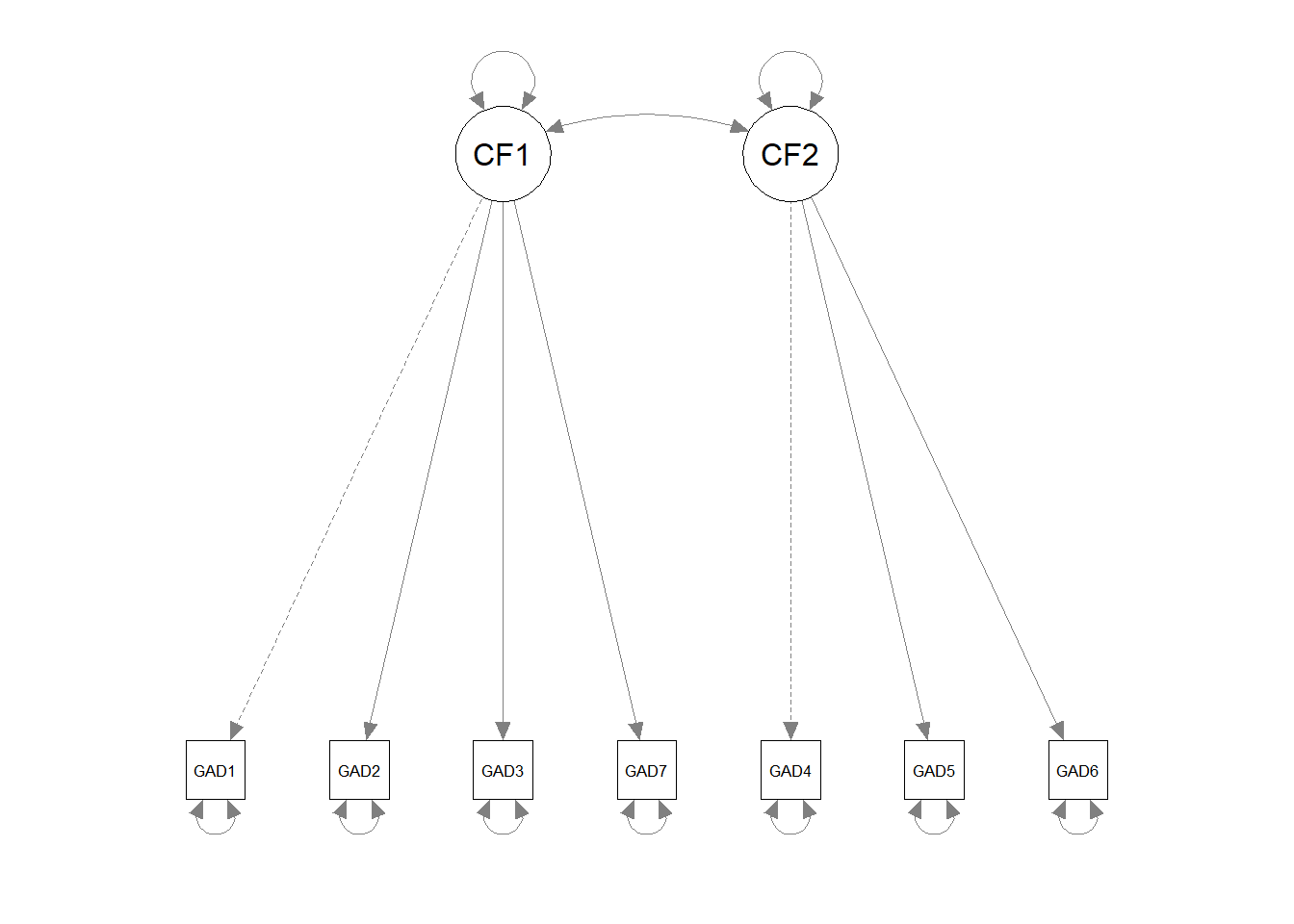
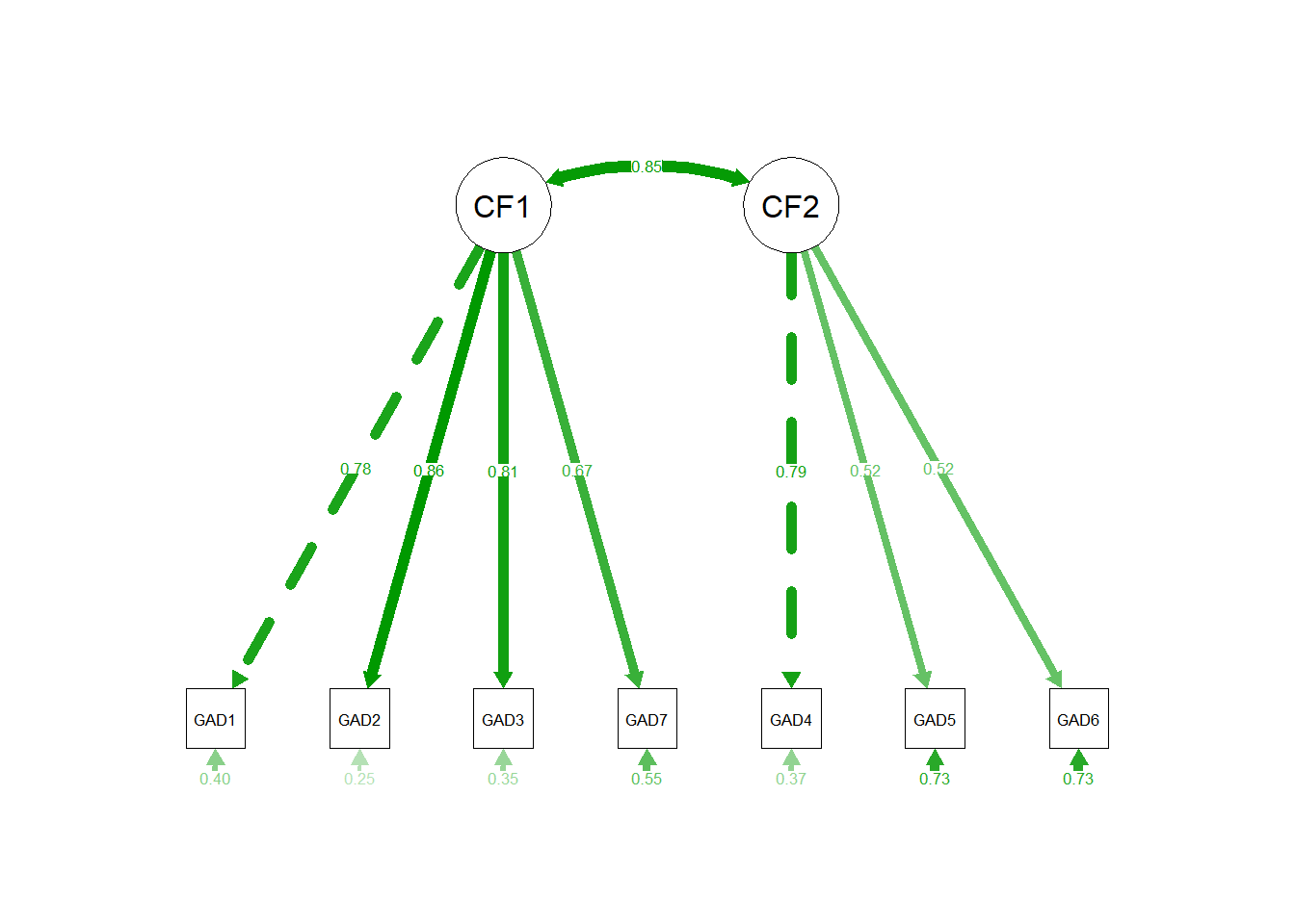
Exercise E1. There exist mutliple packages to visualize your CFA/SEM model from a {lavaan} output, e.g. lavaanPlot::lavaanPlot, see here, and semPlot::semPaths(), see here. Create a visualization of one or multiple of the factor models, just to get a feeling for how this might look.

Show Solution

semPlot::semPaths():

# simple example
semPaths(gad_2f)

# add parameters
semPaths(gad_2f, 'std', 'std', style = "lisrel")

lavaanPlot::lavaanPlot():

# simple example
lavaanPlot(gad_2f)
# add parameters
lavaanPlot(gad_2f, coefs = TRUE, stand = TRUE, covs = TRUE)

F – Ordinal Data

Exercise F1. So far, we have used maximum likelihood estimation. As the items were assessed on a four-point Likert scale, it makes sense to treat the responses as ordinal. To account for this, refit the two-factor model, but with out the freed parameters, and set the argument ordered = TRUE in the cfa() function. This will automatically adjust the estimator. Save the output as gad_2f_ord.

Show Solution

model <- '
  CF1 =~ GAD1 + GAD2 + GAD3 + GAD7
  CF2 =~ GAD4 + GAD5 + GAD6
'
gad_2f_ord <- cfa(model, data = gad7, ordered = TRUE)

Exercise F2. Evaluate the gad_2f_ord model.

Show Solution

summary(gad_2f_ord, fit.measures = TRUE, standardized = TRUE)
lavaan 0.6-19 ended normally after 18 iterations

  Estimator                                       DWLS
  Optimization method                           NLMINB
  Number of model parameters                        29

  Number of observations                         13464

Model Test User Model:
                                              Standard      Scaled
  Test Statistic                               239.844     532.259
  Degrees of freedom                                13          13
  P-value (Chi-square)                           0.000       0.000
  Scaling correction factor                                  0.451
  Shift parameter                                            0.616
    simple second-order correction                                

Model Test Baseline Model:

  Test statistic                            165963.072   95916.802
  Degrees of freedom                                21          21
  P-value                                        0.000       0.000
  Scaling correction factor                                  1.730

User Model versus Baseline Model:

  Comparative Fit Index (CFI)                    0.999       0.995
  Tucker-Lewis Index (TLI)                       0.998       0.991
                                                                  
  Robust Comparative Fit Index (CFI)                         0.981
  Robust Tucker-Lewis Index (TLI)                            0.969

Root Mean Square Error of Approximation:

  RMSEA                                          0.036       0.054
  90 Percent confidence interval - lower         0.032       0.051
  90 Percent confidence interval - upper         0.040       0.058
  P-value H_0: RMSEA <= 0.050                    1.000       0.030
  P-value H_0: RMSEA >= 0.080                    0.000       0.000
                                                                  
  Robust RMSEA                                               0.077
  90 Percent confidence interval - lower                     0.071
  90 Percent confidence interval - upper                     0.083
  P-value H_0: Robust RMSEA <= 0.050                         0.000
  P-value H_0: Robust RMSEA >= 0.080                         0.213

Standardized Root Mean Square Residual:

  SRMR                                           0.025       0.025

Parameter Estimates:

  Parameterization                               Delta
  Standard errors                           Robust.sem
  Information                                 Expected
  Information saturated (h1) model        Unstructured

Latent Variables:
                   Estimate  Std.Err  z-value  P(>|z|)   Std.lv  Std.all
  CF1 =~                                                                
    GAD1              1.000                               0.825    0.825
    GAD2              1.123    0.006  177.510    0.000    0.926    0.926
    GAD3              1.038    0.006  179.478    0.000    0.856    0.856
    GAD7              0.913    0.007  123.662    0.000    0.753    0.753
  CF2 =~                                                                
    GAD4              1.000                               0.853    0.853
    GAD5              0.701    0.011   62.201    0.000    0.598    0.598
    GAD6              0.678    0.010   67.327    0.000    0.579    0.579

Covariances:
                   Estimate  Std.Err  z-value  P(>|z|)   Std.lv  Std.all
  CF1 ~~                                                                
    CF2               0.605    0.006  102.278    0.000    0.860    0.860

Thresholds:
                   Estimate  Std.Err  z-value  P(>|z|)   Std.lv  Std.all
    GAD1|t1          -0.194    0.011  -17.880    0.000   -0.194   -0.194
    GAD1|t2           0.847    0.012   68.692    0.000    0.847    0.847
    GAD1|t3           1.369    0.015   88.787    0.000    1.369    1.369
    GAD2|t1           0.165    0.011   15.230    0.000    0.165    0.165
    GAD2|t2           0.959    0.013   74.837    0.000    0.959    0.959
    GAD2|t3           1.474    0.016   90.095    0.000    1.474    1.474
    GAD3|t1          -0.266    0.011  -24.326    0.000   -0.266   -0.266
    GAD3|t2           0.658    0.012   56.258    0.000    0.658    0.658
    GAD3|t3           1.251    0.015   86.197    0.000    1.251    1.251
    GAD7|t1           0.324    0.011   29.456    0.000    0.324    0.324
    GAD7|t2           1.024    0.013   77.962    0.000    1.024    1.024
    GAD7|t3           1.530    0.017   90.425    0.000    1.530    1.530
    GAD4|t1           0.074    0.011    6.842    0.000    0.074    0.074
    GAD4|t2           0.908    0.013   72.120    0.000    0.908    0.908
    GAD4|t3           1.465    0.016   90.016    0.000    1.465    1.465
    GAD5|t1           0.484    0.011   42.969    0.000    0.484    0.484
    GAD5|t2           1.162    0.014   83.473    0.000    1.162    1.162
    GAD5|t3           1.632    0.018   90.377    0.000    1.632    1.632
    GAD6|t1          -0.253    0.011  -23.175    0.000   -0.253   -0.253
    GAD6|t2           0.742    0.012   62.048    0.000    0.742    0.742
    GAD6|t3           1.392    0.016   89.155    0.000    1.392    1.392

Variances:
                   Estimate  Std.Err  z-value  P(>|z|)   Std.lv  Std.all
   .GAD1              0.320                               0.320    0.320
   .GAD2              0.143                               0.143    0.143
   .GAD3              0.268                               0.268    0.268
   .GAD7              0.433                               0.433    0.433
   .GAD4              0.272                               0.272    0.272
   .GAD5              0.642                               0.642    0.642
   .GAD6              0.665                               0.665    0.665
    CF1               0.680    0.007  102.668    0.000    1.000    1.000
    CF2               0.728    0.010   72.363    0.000    1.000    1.000

The global fit is very good, however, note that the standard fit indices are likely not interpretable by the same standards as when ML-estimation was used. (e.g., Savalei, 2021; Shi & Maydeu-Olivares, 2020; Xia & Yang, 2019). Therefore you should look at the Scaled statistics in the output. These still point towards an acceptable to good global fit.

Local fit – Residual matrix:

lavResiduals(gad_2f_ord)
$type
[1] "cor.bentler"

$cov
       GAD1   GAD2   GAD3   GAD7   GAD4   GAD5   GAD6
GAD1  0.000                                          
GAD2  0.008  0.000                                   
GAD3 -0.026  0.015  0.000                            
GAD7 -0.017 -0.017  0.000  0.000                     
GAD4  0.021 -0.018  0.004  0.011  0.000              
GAD5  0.009 -0.043 -0.044  0.024  0.019  0.000       
GAD6  0.023 -0.042 -0.009  0.062 -0.041  0.042  0.000

$mean
GAD1 GAD2 GAD3 GAD7 GAD4 GAD5 GAD6 
   0    0    0    0    0    0    0 

$th
GAD1|t1 GAD1|t2 GAD1|t3 GAD2|t1 GAD2|t2 GAD2|t3 GAD3|t1 GAD3|t2 GAD3|t3 GAD7|t1 
      0       0       0       0       0       0       0       0       0       0 
GAD7|t2 GAD7|t3 GAD4|t1 GAD4|t2 GAD4|t3 GAD5|t1 GAD5|t2 GAD5|t3 GAD6|t1 GAD6|t2 
      0       0       0       0       0       0       0       0       0       0 
GAD6|t3 
      0 

$cov.z
        GAD1    GAD2    GAD3    GAD7    GAD4    GAD5    GAD6
GAD1   0.000                                                
GAD2   4.360   0.000                                        
GAD3 -10.741  10.905   0.000                                
GAD7  -4.358  -5.955   0.060   0.000                        
GAD4   6.026  -6.739   1.427   2.398   0.000                
GAD5   1.760  -9.373  -8.952   3.657   4.370   0.000        
GAD6   4.896  -9.893  -1.904  10.262 -10.381   6.174   0.000

$mean.z
GAD1 GAD2 GAD3 GAD7 GAD4 GAD5 GAD6 <NA> <NA> <NA> <NA> <NA> <NA> <NA> <NA> <NA> 
   0    0    0    0    0    0    0   NA   NA   NA   NA   NA   NA   NA   NA   NA 
<NA> <NA> <NA> <NA> <NA> 
  NA   NA   NA   NA   NA 

$th.z
GAD1|t1 GAD1|t2 GAD1|t3 GAD2|t1 GAD2|t2 GAD2|t3 GAD3|t1 GAD3|t2 GAD3|t3 GAD7|t1 
      0       0       0       0       0       0       0       0       0       0 
GAD7|t2 GAD7|t3 GAD4|t1 GAD4|t2 GAD4|t3 GAD5|t1 GAD5|t2 GAD5|t3 GAD6|t1 GAD6|t2 
      0       0       0       0       0       0       0       0       0       0 
GAD6|t3 
      0 

$summary
                            cor thresholds    total
srmr                      0.025       0.00    0.019
srmr.se                   0.001         NA    0.001
srmr.exactfit.z          25.709         NA   25.709
srmr.exactfit.pvalue      0.000         NA    0.000
usrmr                     0.024       0.00    0.018
usrmr.se                  0.001         NA    0.000
usrmr.ci.lower            0.022         NA    0.018
usrmr.ci.upper            0.026         NA    0.019
usrmr.closefit.h0.value   0.050       0.05    0.050
usrmr.closefit.z        -20.867         NA -337.361
usrmr.closefit.pvalue     1.000         NA    1.000

The correlation-based residuals are all clearly below .1. The standardized residuals (z-values) are still relatively large. Note that the output contains more information, as the model now also estimated thresholds assumend to be used for the discretization.

Local fit – MI/EPC:

modindices(gad_2f_ord, sort = TRUE, maximum.number = 10)
    lhs op  rhs     mi    epc sepc.lv sepc.all sepc.nox
59  CF2 =~ GAD2 75.558  0.371   0.317    0.317    0.317
79 GAD7 ~~ GAD6 59.581 -0.078  -0.078   -0.145   -0.145
68 GAD2 ~~ GAD3 58.603 -0.063  -0.063   -0.323   -0.323
81 GAD4 ~~ GAD6 55.456  0.096   0.096    0.227    0.227
56  CF1 =~ GAD5 55.456  0.469   0.387    0.387    0.387
61  CF2 =~ GAD7 44.552 -0.279  -0.238   -0.238   -0.238
63 GAD1 ~~ GAD3 41.108  0.054   0.054    0.183    0.183
72 GAD2 ~~ GAD6 31.151  0.059   0.059    0.190    0.190
58  CF2 =~ GAD1 30.869 -0.215  -0.183   -0.183   -0.183
75 GAD3 ~~ GAD5 27.817  0.059   0.059    0.142    0.142

MIs are Still large, but smaller than when ML-estimation was used.

Parameters:

lavInspect(gad_2f_ord, what = "std.all")$lambda ^2
       CF1   CF2
GAD1 0.680 0.000
GAD2 0.857 0.000
GAD3 0.732 0.000
GAD7 0.567 0.000
GAD4 0.000 0.728
GAD5 0.000 0.358
GAD6 0.000 0.335

Communalities are larger than when ML-estimation is used. Communalities of items GAD5 and GAD6 now come closer to the conventional threshold of .4.

Overall evaluation:

Both global and local model fit are better than when ML-estimation is used.

G – Handling Missing Values

Exercise G1. So far, we have used {lavaan}s default handling of missing values, which is list-wise deletion. Refit the model using full information maximum likelihood (FIML) / direct ML estimation to impute missing values by adding the argument missing = "ml" (aliases are "fiml" or "direct", so you might come across these in other {lavaan} syntax). Look at the solution.

Show Solution

model <- '
  CF1 =~ GAD1 + GAD2 + GAD3 + GAD7
  CF2 =~ GAD4 + GAD5 + GAD6
'
gad_2f_fiml <- cfa(model, data = gad7, missing = "ml")

summary(gad_2f_fiml, fit.measures = TRUE, standardized = TRUE)
lavaan 0.6-19 ended normally after 25 iterations

  Estimator                                         ML
  Optimization method                           NLMINB
  Number of model parameters                        22

  Number of observations                         13464
  Number of missing patterns                         1

Model Test User Model:
                                                      
  Test statistic                               567.321
  Degrees of freedom                                13
  P-value (Chi-square)                           0.000

Model Test Baseline Model:

  Test statistic                             38698.973
  Degrees of freedom                                21
  P-value                                        0.000

User Model versus Baseline Model:

  Comparative Fit Index (CFI)                    0.986
  Tucker-Lewis Index (TLI)                       0.977
                                                      
  Robust Comparative Fit Index (CFI)             0.986
  Robust Tucker-Lewis Index (TLI)                0.977

Loglikelihood and Information Criteria:

  Loglikelihood user model (H0)            -106264.271
  Loglikelihood unrestricted model (H1)    -105980.610
                                                      
  Akaike (AIC)                              212572.542
  Bayesian (BIC)                            212737.713
  Sample-size adjusted Bayesian (SABIC)     212667.799

Root Mean Square Error of Approximation:

  RMSEA                                          0.056
  90 Percent confidence interval - lower         0.052
  90 Percent confidence interval - upper         0.060
  P-value H_0: RMSEA <= 0.050                    0.004
  P-value H_0: RMSEA >= 0.080                    0.000
                                                      
  Robust RMSEA                                   0.056
  90 Percent confidence interval - lower         0.052
  90 Percent confidence interval - upper         0.060
  P-value H_0: Robust RMSEA <= 0.050             0.004
  P-value H_0: Robust RMSEA >= 0.080             0.000

Standardized Root Mean Square Residual:

  SRMR                                           0.021

Parameter Estimates:

  Standard errors                             Standard
  Information                                 Observed
  Observed information based on                Hessian

Latent Variables:
                   Estimate  Std.Err  z-value  P(>|z|)   Std.lv  Std.all
  CF1 =~                                                                
    GAD1              1.000                               0.718    0.775
    GAD2              1.102    0.011  103.903    0.000    0.792    0.865
    GAD3              1.103    0.012   95.430    0.000    0.793    0.807
    GAD7              0.835    0.011   77.964    0.000    0.600    0.671
  CF2 =~                                                                
    GAD4              1.000                               0.731    0.793
    GAD5              0.598    0.011   54.613    0.000    0.437    0.522
    GAD6              0.663    0.013   52.640    0.000    0.485    0.521

Covariances:
                   Estimate  Std.Err  z-value  P(>|z|)   Std.lv  Std.all
  CF1 ~~                                                                
    CF2               0.445    0.008   56.646    0.000    0.848    0.848

Intercepts:
                   Estimate  Std.Err  z-value  P(>|z|)   Std.lv  Std.all
   .GAD1              0.861    0.008  107.826    0.000    0.861    0.929
   .GAD2              0.673    0.008   85.326    0.000    0.673    0.735
   .GAD3              0.966    0.008  114.030    0.000    0.966    0.983
   .GAD7              0.589    0.008   76.384    0.000    0.589    0.658
   .GAD4              0.724    0.008   91.132    0.000    0.724    0.785
   .GAD5              0.488    0.007   67.659    0.000    0.488    0.583
   .GAD6              0.911    0.008  113.528    0.000    0.911    0.978

Variances:
                   Estimate  Std.Err  z-value  P(>|z|)   Std.lv  Std.all
   .GAD1              0.342    0.005   66.237    0.000    0.342    0.399
   .GAD2              0.212    0.004   51.113    0.000    0.212    0.252
   .GAD3              0.337    0.005   62.632    0.000    0.337    0.349
   .GAD7              0.440    0.006   73.536    0.000    0.440    0.550
   .GAD4              0.315    0.007   43.053    0.000    0.315    0.370
   .GAD5              0.509    0.007   74.152    0.000    0.509    0.727
   .GAD6              0.632    0.009   74.192    0.000    0.632    0.728
    CF1               0.516    0.010   51.261    0.000    1.000    1.000
    CF2               0.535    0.011   46.688    0.000    1.000    1.000

Exercise G2. When we use the DWLS-estimator, no direct imputation method is available. So here we can use multiple imputation. The {lavaan.mi}-package provides helpful functions to do this. They are named just like their {lavaan}-counterpart, but with a .mi suffix. Refit the model from Exercise F1 but use the cfa.mi() function. Look at the results.

Show Solution

model <- '
  CF1 =~ GAD1 + GAD2 + GAD3 + GAD7
  CF2 =~ GAD4 + GAD5 + GAD6
'


# Impute 5 datasets (common practice)
gad7_imp <- mice(data = gad7 %>% 
                   mutate(across(GAD1:GAD7, ordered)),
                 m = 5, 
                 # Specify imputation method for ordinal data
                 method = c(rep("polr", 7), "midastouch", "midastouch"))

 iter imp variable
  1   1
  1   2
  1   3
  1   4
  1   5
  2   1
  2   2
  2   3
  2   4
  2   5
  3   1
  3   2
  3   3
  3   4
  3   5
  4   1
  4   2
  4   3
  4   4
  4   5
  5   1
  5   2
  5   3
  5   4
  5   5
Warning: Number of logged events: 2
gad7_imp <- map(seq_len(5),
                ~complete(gad7_imp, action = .x, inc = FALSE))

gad_2f_ord_imp <- cfa.mi(model, data = gad7_imp, ordered = TRUE)

Exercise G3. Evaluate the gad_2f_ord_imp model.

Show Solution

summary(gad_2f_ord_imp, fit.measures = TRUE, standardized = TRUE)
lavaan.mi object fit to 5 imputed data sets using:
 - lavaan    (0.6-19)
 - lavaan.mi (0.1-0)
See class?lavaan.mi help page for available methods. 

Convergence information:
The model converged on 5 imputed data sets.
Standard errors were available for all imputations.

  Estimator                                       DWLS
  Optimization method                           NLMINB
  Number of model parameters                        29

  Number of observations                         13464

Model Test User Model:

                                                Standard      Scaled
  Test statistic                                 239.844     532.259
  Degrees of freedom                                  13          13
  P-value                                          0.000       0.000
  Average scaling correction factor                            0.451
  Average shift parameter                                      0.616
    simple second-order correction                                  
  Pooling method                                      D2            
    Pooled statistic                          "standard"            
    "scaled.shifted" correction applied            AFTER     pooling

Model Test Baseline Model:

  Test statistic                            165963.072   95916.802
  Degrees of freedom                                21          21
  P-value                                        0.000       0.000
  Scaling correction factor                                  1.730

User Model versus Baseline Model:

  Comparative Fit Index (CFI)                    0.999       0.995
  Tucker-Lewis Index (TLI)                       0.998       0.991
                                                                  
  Robust Comparative Fit Index (CFI)                         0.981
  Robust Tucker-Lewis Index (TLI)                            0.969

Root Mean Square Error of Approximation:

  RMSEA                                          0.036       0.054
  90 Percent confidence interval - lower         0.032       0.051
  90 Percent confidence interval - upper         0.040       0.058
  P-value H_0: RMSEA <= 0.050                    1.000       0.030
  P-value H_0: RMSEA >= 0.080                    0.000       0.000
                                                                  
  Robust RMSEA                                               0.077
  90 Percent confidence interval - lower                     0.071
  90 Percent confidence interval - upper                     0.083
  P-value H_0: Robust RMSEA <= 0.050                         0.000
  P-value H_0: Robust RMSEA >= 0.080                         0.213

Standardized Root Mean Square Residual:

  SRMR                                           0.025       0.025

Parameter Estimates:

  Parameterization                               Delta
  Standard errors                                  Robust.sem
  Information                                        Expected
  Information saturated (h1) model               Unstructured
                                                             
  Pooled across imputations              Rubin's (1987) rules
  Augment within-imputation variance     Scale by average RIV
  Wald test for pooled parameters          t(df) distribution

  Pooled t statistics with df >= 1000 are displayed with
  df = Inf(inity) to save space. Although the t distribution
  with large df closely approximates a standard normal
  distribution, exact df for reporting these t tests can be
  obtained from parameterEstimates.mi() 


Latent Variables:
                   Estimate  Std.Err  t-value       df  P(>|t|)   Std.lv
  CF1 =~                                                                
    GAD1              1.000                                        0.825
    GAD2              1.123    0.006  177.510      Inf    0.000    0.926
    GAD3              1.038    0.006  179.478      Inf    0.000    0.856
    GAD7              0.913    0.007  123.662      Inf    0.000    0.753
  CF2 =~                                                                
    GAD4              1.000                                        0.853
    GAD5              0.701    0.011   62.201      Inf    0.000    0.598
    GAD6              0.678    0.010   67.327      Inf    0.000    0.579
  Std.all
         
    0.825
    0.926
    0.856
    0.753
         
    0.853
    0.598
    0.579

Covariances:
                   Estimate  Std.Err  t-value       df  P(>|t|)   Std.lv
  CF1 ~~                                                                
    CF2               0.605    0.006  102.278      Inf    0.000    0.860
  Std.all
         
    0.860

Thresholds:
                   Estimate  Std.Err  t-value       df  P(>|t|)   Std.lv
    GAD1|t1          -0.194    0.011  -17.880      Inf    0.000   -0.194
    GAD1|t2           0.847    0.012   68.692      Inf    0.000    0.847
    GAD1|t3           1.369    0.015   88.787      Inf    0.000    1.369
    GAD2|t1           0.165    0.011   15.230      Inf    0.000    0.165
    GAD2|t2           0.959    0.013   74.837      Inf    0.000    0.959
    GAD2|t3           1.474    0.016   90.095      Inf    0.000    1.474
    GAD3|t1          -0.266    0.011  -24.326      Inf    0.000   -0.266
    GAD3|t2           0.658    0.012   56.258      Inf    0.000    0.658
    GAD3|t3           1.251    0.015   86.197      Inf    0.000    1.251
    GAD7|t1           0.324    0.011   29.456      Inf    0.000    0.324
    GAD7|t2           1.024    0.013   77.962      Inf    0.000    1.024
    GAD7|t3           1.530    0.017   90.425      Inf    0.000    1.530
    GAD4|t1           0.074    0.011    6.842      Inf    0.000    0.074
    GAD4|t2           0.908    0.013   72.120      Inf    0.000    0.908
    GAD4|t3           1.465    0.016   90.016      Inf    0.000    1.465
    GAD5|t1           0.484    0.011   42.969      Inf    0.000    0.484
    GAD5|t2           1.162    0.014   83.473      Inf    0.000    1.162
    GAD5|t3           1.632    0.018   90.377      Inf    0.000    1.632
    GAD6|t1          -0.253    0.011  -23.175      Inf    0.000   -0.253
    GAD6|t2           0.742    0.012   62.048      Inf    0.000    0.742
    GAD6|t3           1.392    0.016   89.155      Inf    0.000    1.392
  Std.all
   -0.194
    0.847
    1.369
    0.165
    0.959
    1.474
   -0.266
    0.658
    1.251
    0.324
    1.024
    1.530
    0.074
    0.908
    1.465
    0.484
    1.162
    1.632
   -0.253
    0.742
    1.392

Variances:
                   Estimate  Std.Err  t-value       df  P(>|t|)   Std.lv
   .GAD1              0.320                                        0.320
   .GAD2              0.143                                        0.143
   .GAD3              0.268                                        0.268
   .GAD7              0.433                                        0.433
   .GAD4              0.272                                        0.272
   .GAD5              0.642                                        0.642
   .GAD6              0.665                                        0.665
    CF1               0.680    0.007  102.668      Inf    0.000    1.000
    CF2               0.728    0.010   72.363      Inf    0.000    1.000
  Std.all
    0.320
    0.143
    0.268
    0.433
    0.272
    0.642
    0.665
    1.000
    1.000

H – Measurement Invariance

Exercise H1. An important question is whether a measurement model is invariant across groups, i.e., whether the same model structure and parameters apply to all groups (e.g. across genders). When would a non-invariance occur? For example, if women would tend to agree to some items more than men, not because they have higher values in their true latent anxiety score, but because it is socially more acceptable/less stigmatized behavior in women than in men. Test the configural, weak, strong, and strict factorial invariance across genders for the gad_2f_fiml model, using the group.equal argument of cfa() (see also lavaan group comparison tutorial). Compare the models using an LRT (lavTestLRT()).

Show Solution

model <- '
  CF1 =~ GAD1 + GAD2 + GAD3 + GAD7
  CF2 =~ GAD4 + GAD5 + GAD6
'

# configural invariance
gad7_2f_conf <- cfa(model, data = gad7, missing = "ml", group = "Gender")

# weak invariance
gad7_2f_weak <- cfa(model, data = gad7, missing = "ml", group = "Gender",
                    group.equal = "loadings")

# strong invariance
gad7_2f_strong <- cfa(model, data = gad7, missing = "ml", group = "Gender",
                      group.equal = c("intercepts", "loadings"))

# strict invariance
gad7_2f_strict <- cfa(model, data = gad7, missing = "ml", group = "Gender",
                      group.equal = c("residuals", "intercepts", "loadings"))

# model comparison tests
lavTestLRT(gad7_2f_conf, gad7_2f_weak, gad7_2f_strong, gad7_2f_strict)

Chi-Squared Difference Test

               Df    AIC    BIC  Chisq Chisq diff    RMSEA Df diff Pr(>Chisq)
gad7_2f_conf   39 212204 212700 626.64                                       
gad7_2f_weak   49 212216 212636 658.38     31.745 0.022012      10  0.0004415
gad7_2f_strong 59 212220 212565 682.69     24.312 0.017858      10  0.0068130
gad7_2f_strict 73 212235 212475 725.72     43.027 0.021494      14  8.481e-05
                  
gad7_2f_conf      
gad7_2f_weak   ***
gad7_2f_strong ** 
gad7_2f_strict ***
---
Signif. codes:  0 '***' 0.001 '**' 0.01 '*' 0.05 '.' 0.1 ' ' 1

The LRT sequentially compares the models to each other. According to these tests, no invariance is supported. But given the high sample-size this is again unsurprising. In such a situation, we can also look at differences in fit indeces (see Chen, 2007 for details). Remeber, cut-offs for \(\Delta\) fit indices, according to Chen (2007) are:

  • Loadings invariant if: \(\Delta CFI \leq -.005\) and \(\Delta RMSEA \geq .010\) or \(\Delta SRMR \geq .025\)
  • Intercept or residuals invariant if: \(\Delta CFI \leq -.005\) and \(\Delta RMSEA \geq .010\) or \(\Delta SRMR \geq .005\)

Let’s look at the \(\Delta\) fit indices:

fit_ind_conf <- fitMeasures(gad7_2f_conf)[c("cfi", "rmsea", "srmr")]
fit_ind_weak <- fitMeasures(gad7_2f_weak)[c("cfi", "rmsea", "srmr")]
fit_ind_strong <- fitMeasures(gad7_2f_strong)[c("cfi", "rmsea", "srmr")]
fit_ind_strict <- fitMeasures(gad7_2f_strict)[c("cfi", "rmsea", "srmr")]

# delta for weak
round(fit_ind_conf - fit_ind_weak, 3)
   cfi  rmsea   srmr 
 0.001  0.005 -0.001 
# delta for strong
round(fit_ind_weak - fit_ind_strong, 3)
  cfi rmsea  srmr 
0.000 0.004 0.000 
# delta for strict
round(fit_ind_strong - fit_ind_strict, 3)
   cfi  rmsea   srmr 
 0.001  0.004 -0.001 

According to the \(\Delta\) fit indices we have invariance across the groups.

We can look at the solutions across groups by inspecting the summary of gad7_2f_conf:

summary(gad7_2f_conf, fit.measures = TRUE, standardized = TRUE)
lavaan 0.6-19 ended normally after 175 iterations

  Estimator                                         ML
  Optimization method                           NLMINB
  Number of model parameters                        66

  Number of observations per group:                   
    Male                                         12699
    Female                                         713
    Other                                           52
  Number of missing patterns per group:               
    Male                                             1
    Female                                           1
    Other                                            1

Model Test User Model:
                                                      
  Test statistic                               626.636
  Degrees of freedom                                39
  P-value (Chi-square)                           0.000
  Test statistic for each group:
    Male                                       534.617
    Female                                      50.201
    Other                                       41.818

Model Test Baseline Model:

  Test statistic                             37962.343
  Degrees of freedom                                63
  P-value                                        0.000

User Model versus Baseline Model:

  Comparative Fit Index (CFI)                    0.984
  Tucker-Lewis Index (TLI)                       0.975
                                                      
  Robust Comparative Fit Index (CFI)             0.984
  Robust Tucker-Lewis Index (TLI)                0.975

Loglikelihood and Information Criteria:

  Loglikelihood user model (H0)            -106036.026
  Loglikelihood unrestricted model (H1)    -105722.708
                                                      
  Akaike (AIC)                              212204.052
  Bayesian (BIC)                            212699.566
  Sample-size adjusted Bayesian (SABIC)     212489.824

Root Mean Square Error of Approximation:

  RMSEA                                          0.058
  90 Percent confidence interval - lower         0.054
  90 Percent confidence interval - upper         0.062
  P-value H_0: RMSEA <= 0.050                    0.001
  P-value H_0: RMSEA >= 0.080                    0.000
                                                      
  Robust RMSEA                                   0.058
  90 Percent confidence interval - lower         0.054
  90 Percent confidence interval - upper         0.062
  P-value H_0: Robust RMSEA <= 0.050             0.001
  P-value H_0: Robust RMSEA >= 0.080             0.000

Standardized Root Mean Square Residual:

  SRMR                                           0.021

Parameter Estimates:

  Standard errors                             Standard
  Information                                 Observed
  Observed information based on                Hessian


Group 1 [Male]:

Latent Variables:
                   Estimate  Std.Err  z-value  P(>|z|)   Std.lv  Std.all
  CF1 =~                                                                
    GAD1              1.000                               0.700    0.768
    GAD2              1.096    0.011   97.871    0.000    0.767    0.857
    GAD3              1.114    0.012   90.360    0.000    0.779    0.802
    GAD7              0.832    0.011   73.723    0.000    0.582    0.663
  CF2 =~                                                                
    GAD4              1.000                               0.714    0.786
    GAD5              0.599    0.012   51.747    0.000    0.427    0.516
    GAD6              0.669    0.013   50.021    0.000    0.477    0.516

Covariances:
                   Estimate  Std.Err  z-value  P(>|z|)   Std.lv  Std.all
  CF1 ~~                                                                
    CF2               0.421    0.008   54.208    0.000    0.844    0.844

Intercepts:
                   Estimate  Std.Err  z-value  P(>|z|)   Std.lv  Std.all
   .GAD1              0.834    0.008  103.223    0.000    0.834    0.916
   .GAD2              0.643    0.008   81.082    0.000    0.643    0.720
   .GAD3              0.940    0.009  109.021    0.000    0.940    0.967
   .GAD7              0.569    0.008   72.971    0.000    0.569    0.648
   .GAD4              0.700    0.008   86.879    0.000    0.700    0.771
   .GAD5              0.478    0.007   65.032    0.000    0.478    0.577
   .GAD6              0.896    0.008  109.133    0.000    0.896    0.968

Variances:
                   Estimate  Std.Err  z-value  P(>|z|)   Std.lv  Std.all
   .GAD1              0.340    0.005   64.265    0.000    0.340    0.410
   .GAD2              0.212    0.004   50.151    0.000    0.212    0.265
   .GAD3              0.336    0.006   60.477    0.000    0.336    0.356
   .GAD7              0.433    0.006   71.372    0.000    0.433    0.561
   .GAD4              0.316    0.007   42.154    0.000    0.316    0.383
   .GAD5              0.504    0.007   71.949    0.000    0.504    0.734
   .GAD6              0.627    0.009   71.926    0.000    0.627    0.733
    CF1               0.489    0.010   48.967    0.000    1.000    1.000
    CF2               0.509    0.011   44.333    0.000    1.000    1.000


Group 2 [Female]:

Latent Variables:
                   Estimate  Std.Err  z-value  P(>|z|)   Std.lv  Std.all
  CF1 =~                                                                
    GAD1              1.000                               0.842    0.802
    GAD2              1.186    0.042   28.380    0.000    0.999    0.916
    GAD3              1.048    0.042   24.967    0.000    0.882    0.834
    GAD7              0.903    0.044   20.719    0.000    0.760    0.720
  CF2 =~                                                                
    GAD4              1.000                               0.869    0.846
    GAD5              0.603    0.041   14.587    0.000    0.524    0.565
    GAD6              0.583    0.046   12.765    0.000    0.507    0.519

Covariances:
                   Estimate  Std.Err  z-value  P(>|z|)   Std.lv  Std.all
  CF1 ~~                                                                
    CF2               0.626    0.045   13.934    0.000    0.855    0.855

Intercepts:
                   Estimate  Std.Err  z-value  P(>|z|)   Std.lv  Std.all
   .GAD1              1.278    0.039   32.473    0.000    1.278    1.216
   .GAD2              1.157    0.041   28.357    0.000    1.157    1.062
   .GAD3              1.388    0.040   35.059    0.000    1.388    1.313
   .GAD7              0.903    0.040   22.821    0.000    0.903    0.855
   .GAD4              1.088    0.038   28.271    0.000    1.088    1.059
   .GAD5              0.630    0.035   18.116    0.000    0.630    0.678
   .GAD6              1.153    0.037   31.561    0.000    1.153    1.182

Variances:
                   Estimate  Std.Err  z-value  P(>|z|)   Std.lv  Std.all
   .GAD1              0.395    0.025   15.806    0.000    0.395    0.358
   .GAD2              0.190    0.019   10.013    0.000    0.190    0.160
   .GAD3              0.340    0.023   14.985    0.000    0.340    0.304
   .GAD7              0.539    0.032   17.076    0.000    0.539    0.482
   .GAD4              0.301    0.035    8.694    0.000    0.301    0.285
   .GAD5              0.587    0.034   17.113    0.000    0.587    0.681
   .GAD6              0.695    0.040   17.413    0.000    0.695    0.730
    CF1               0.709    0.056   12.600    0.000    1.000    1.000
    CF2               0.756    0.062   12.223    0.000    1.000    1.000


Group 3 [Other]:

Latent Variables:
                   Estimate  Std.Err  z-value  P(>|z|)   Std.lv  Std.all
  CF1 =~                                                                
    GAD1              1.000                               1.077    0.924
    GAD2              1.068    0.104   10.239    0.000    1.150    0.896
    GAD3              0.969    0.096   10.090    0.000    1.044    0.882
    GAD7              0.833    0.133    6.247    0.000    0.897    0.714
  CF2 =~                                                                
    GAD4              1.000                               1.017    0.847
    GAD5              0.906    0.151    6.013    0.000    0.922    0.790
    GAD6              0.912    0.160    5.685    0.000    0.928    0.747

Covariances:
                   Estimate  Std.Err  z-value  P(>|z|)   Std.lv  Std.all
  CF1 ~~                                                                
    CF2               0.927    0.232    3.996    0.000    0.845    0.845

Intercepts:
                   Estimate  Std.Err  z-value  P(>|z|)   Std.lv  Std.all
   .GAD1              1.712    0.162   10.586    0.000    1.712    1.468
   .GAD2              1.346    0.178    7.558    0.000    1.346    1.048
   .GAD3              1.558    0.164    9.491    0.000    1.558    1.316
   .GAD7              1.135    0.174    6.513    0.000    1.135    0.903
   .GAD4              1.500    0.167    9.007    0.000    1.500    1.249
   .GAD5              0.942    0.162    5.822    0.000    0.942    0.807
   .GAD6              1.385    0.172    8.035    0.000    1.385    1.114

Variances:
                   Estimate  Std.Err  z-value  P(>|z|)   Std.lv  Std.all
   .GAD1              0.198    0.065    3.061    0.002    0.198    0.146
   .GAD2              0.326    0.094    3.463    0.001    0.326    0.198
   .GAD3              0.311    0.084    3.709    0.000    0.311    0.222
   .GAD7              0.773    0.170    4.557    0.000    0.773    0.490
   .GAD4              0.407    0.129    3.152    0.002    0.407    0.282
   .GAD5              0.512    0.138    3.712    0.000    0.512    0.376
   .GAD6              0.683    0.168    4.073    0.000    0.683    0.442
    CF1               1.161    0.269    4.319    0.000    1.000    1.000
    CF2               1.035    0.290    3.572    0.000    1.000    1.000

The parameter estimates do look quite different across models. Note the low N for Gender == "other", thus this solution is likely unstable.

I – Higher-Order Models

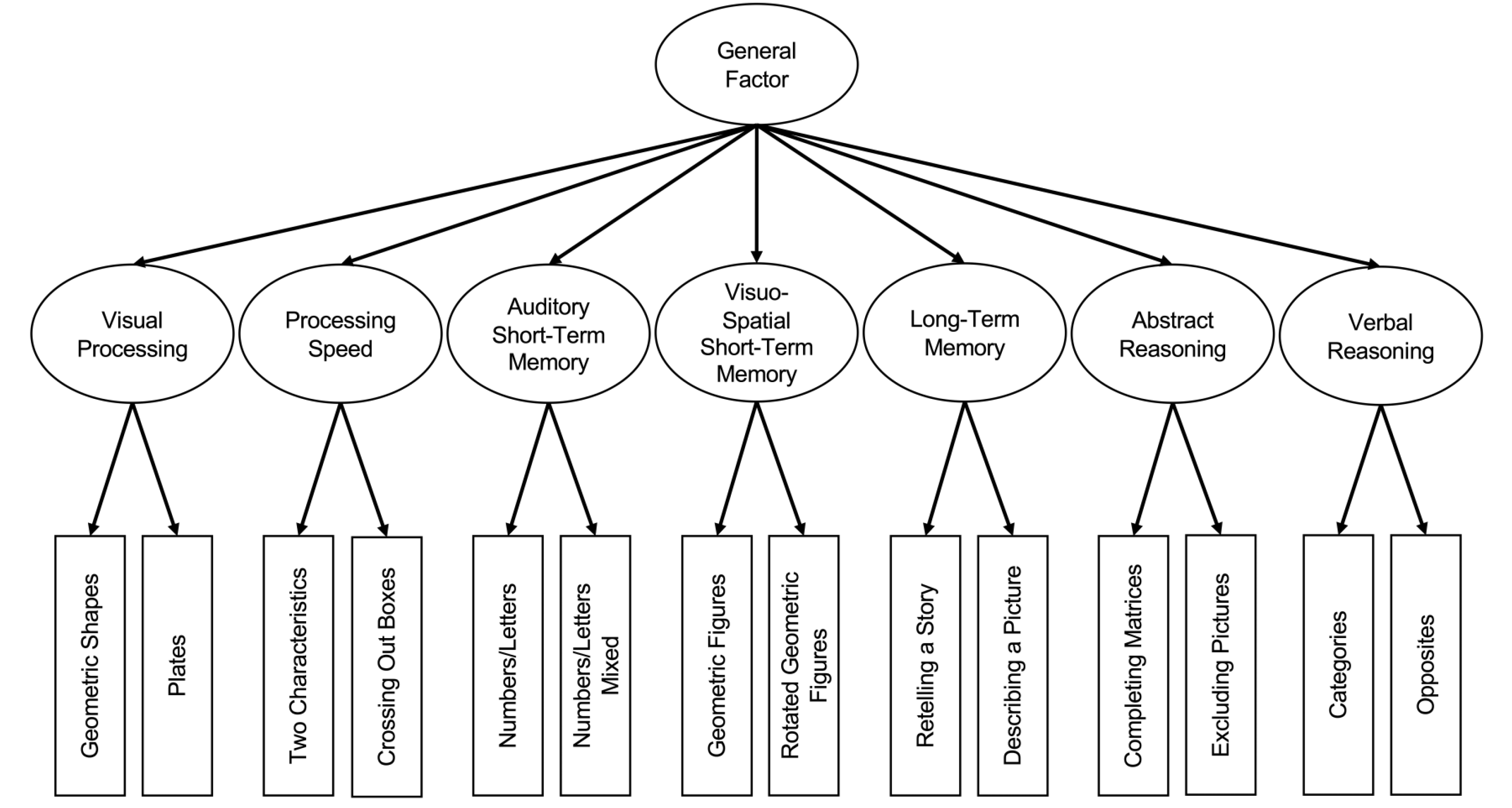
Sometimes, we have multiple latent factors and want to model their covariances with a higher-order factor. Probably the most prominent example is intelligence tests, where we have multiple subtests per group factor and then a general factor on top. While we have no raw-data available, but given a correlation matrix and SDs, we can compute the covariance matrix and run the CFA with this. This means that if you see a paper and want to replicate the analyses, you can do so given the correlation matrix, SD vector, and sample size (and mean vector, if the mean structure is needed). The EFAtools package contains the IDS2_R data, which is the correlation matrix among subtests of the intelligence and development scales - 2 used in Grieder & Grob (2020). This matrix is based on the standardihzation and validation sample of N = 1991 children and adolescents aged 5 to 20 years. They also report the SDs in their paper, copy the code below to get the correlation matrix and SDs:

IDS2_R <- EFAtools::IDS2_R
IDS2_SD <- c(3.20, 3.18, 3.13, 3.15, 3.20, 3.11, 3.06, 3.07, 3.14, 3.18, 3.22,
             3.16, 3.16, 3.08)
N_sample <- 1991

Exercise I1. Compute the covariance matrix IDS2_S from the information above, once using the {lavaan} cor2cov() function and once by hand: \(DRD\), where \(D\) is the diagonal matrix of the SDs and \(R\) is the correlation matrix. Do the two matrices match?

Show Solution

(IDS2_S_hand <- diag(IDS2_SD) %*% IDS2_R %*% diag(IDS2_SD))
           [,1]      [,2]     [,3]     [,4]      [,5]     [,6]     [,7]
 [1,] 10.240000  4.081717 3.536396 4.357584  3.975157 3.585440 3.009052
 [2,]  4.081717 10.112400 2.596806 2.786070  3.010340 2.891668 2.255522
 [3,]  3.536396  2.596806 9.796900 6.149935  3.547104 3.226522 2.515978
 [4,]  4.357584  2.786070 6.149935 9.922500  3.379811 2.983872 2.554413
 [5,]  3.975157  3.010340 3.547104 3.379811 10.240000 7.711421 3.297052
 [6,]  3.585440  2.891668 3.226522 2.983872  7.711421 9.672100 3.042057
 [7,]  3.009052  2.255522 2.515978 2.554413  3.297052 3.042057 9.363600
 [8,]  3.396517  2.835043 2.953441 3.161878  3.616297 3.647863 4.944911
 [9,]  4.676871  3.589468 3.746134 3.781784  3.970166 3.602882 3.271122
[10,]  3.908343  3.024658 3.106926 3.198629  3.792417 3.311587 2.936031
[11,]  4.188298  2.758298 3.281371 3.191953  4.452323 4.106888 2.776077
[12,]  4.038054  2.812217 3.298363 3.222231  4.687267 4.406760 2.762350
[13,]  3.139629  2.559401 3.302834 3.082766  3.710342 3.729285 2.797975
[14,]  1.794384  2.131756 2.288278 2.128361  2.072583 2.151967 2.302367
          [,8]     [,9]     [,10]     [,11]    [,12]    [,13]    [,14]
 [1,] 3.396517 4.676871  3.908343  4.188298 4.038054 3.139629 1.794384
 [2,] 2.835043 3.589468  3.024658  2.758298 2.812217 2.559401 2.131756
 [3,] 2.953441 3.746134  3.106926  3.281371 3.298363 3.302834 2.288278
 [4,] 3.161878 3.781784  3.198629  3.191953 3.222231 3.082766 2.128361
 [5,] 3.616297 3.970166  3.792417  4.452323 4.687267 3.710342 2.072583
 [6,] 3.647863 3.602882  3.311587  4.106888 4.406760 3.729285 2.151967
 [7,] 4.944911 3.271122  2.936031  2.776077 2.762350 2.797975 2.302367
 [8,] 9.424900 3.877069  3.400261  3.057707 3.328200 3.161026 2.763804
 [9,] 3.877069 9.859600  4.405084  3.973105 3.776185 3.580439 2.524304
[10,] 3.400261 4.405084 10.112400  3.774177 3.587428 3.287034 2.485509
[11,] 3.057707 3.973105  3.774177 10.368400 6.386077 4.854906 2.527733
[12,] 3.328200 3.776185  3.587428  6.386077 9.985600 5.093634 2.453077
[13,] 3.161026 3.580439  3.287034  4.854906 5.093634 9.985600 3.893256
[14,] 2.763804 2.524304  2.485509  2.527733 2.453077 3.893256 9.486400
(IDS2_S <- cor2cov(IDS2_R, IDS2_SD))
             GS        PL       TC       CB        NL      NLM       GF
 [1,] 10.240000  4.081717 3.536396 4.357584  3.975157 3.585440 3.009052
 [2,]  4.081717 10.112400 2.596806 2.786070  3.010340 2.891668 2.255522
 [3,]  3.536396  2.596806 9.796900 6.149935  3.547104 3.226522 2.515978
 [4,]  4.357584  2.786070 6.149935 9.922500  3.379811 2.983872 2.554413
 [5,]  3.975157  3.010340 3.547104 3.379811 10.240000 7.711421 3.297052
 [6,]  3.585440  2.891668 3.226522 2.983872  7.711421 9.672100 3.042057
 [7,]  3.009052  2.255522 2.515978 2.554413  3.297052 3.042057 9.363600
 [8,]  3.396517  2.835043 2.953441 3.161878  3.616297 3.647863 4.944911
 [9,]  4.676871  3.589468 3.746134 3.781784  3.970166 3.602882 3.271122
[10,]  3.908343  3.024658 3.106926 3.198629  3.792417 3.311587 2.936031
[11,]  4.188298  2.758298 3.281371 3.191953  4.452323 4.106888 2.776077
[12,]  4.038054  2.812217 3.298363 3.222231  4.687267 4.406760 2.762350
[13,]  3.139629  2.559401 3.302834 3.082766  3.710342 3.729285 2.797975
[14,]  1.794384  2.131756 2.288278 2.128361  2.072583 2.151967 2.302367
           RGF       CM        EP        CA       OP       RS       DP
 [1,] 3.396517 4.676871  3.908343  4.188298 4.038054 3.139629 1.794384
 [2,] 2.835043 3.589468  3.024658  2.758298 2.812217 2.559401 2.131756
 [3,] 2.953441 3.746134  3.106926  3.281371 3.298363 3.302834 2.288278
 [4,] 3.161878 3.781784  3.198629  3.191953 3.222231 3.082766 2.128361
 [5,] 3.616297 3.970166  3.792417  4.452323 4.687267 3.710342 2.072583
 [6,] 3.647863 3.602882  3.311587  4.106888 4.406760 3.729285 2.151967
 [7,] 4.944911 3.271122  2.936031  2.776077 2.762350 2.797975 2.302367
 [8,] 9.424900 3.877069  3.400261  3.057707 3.328200 3.161026 2.763804
 [9,] 3.877069 9.859600  4.405084  3.973105 3.776185 3.580439 2.524304
[10,] 3.400261 4.405084 10.112400  3.774177 3.587428 3.287034 2.485509
[11,] 3.057707 3.973105  3.774177 10.368400 6.386077 4.854906 2.527733
[12,] 3.328200 3.776185  3.587428  6.386077 9.985600 5.093634 2.453077
[13,] 3.161026 3.580439  3.287034  4.854906 5.093634 9.985600 3.893256
[14,] 2.763804 2.524304  2.485509  2.527733 2.453077 3.893256 9.486400

Both return the same result.

Exercise I2. Below is a picture of the theoretical model of the IDS2 (Figure by Grieder & Grob, 2020). Use this picture and the subscale names in IDS2_S (see also ?EFAtools::IDS2_R for the full names) to build and fit a CFA first with only a first-order structure in {lavaan}, i.e., do not yet include a higher order factor (feel free to abbreviate the names of the group factors). To this end, specify the sample.cov and sample.nobs arguments in cfa() with the covariance matrix and the sample size. How does the model fit?

Show Solution

IDS2_model <- "
# group factors
vis_proc =~ GS + PL
proc_spd =~ TC + CB
aud_stm =~ NL + NLM
vsp_stm =~ GF + RGF
ltm =~ RS + DP
abs_rsn =~ CM + EP
vrb_rsn =~ CA + OP
"

IDS2_cfa <- cfa(IDS2_model, sample.cov = IDS2_S, sample.nobs = N_sample)
summary(IDS2_cfa, fit.measures = TRUE, standardized = TRUE)
lavaan 0.6-19 ended normally after 149 iterations

  Estimator                                         ML
  Optimization method                           NLMINB
  Number of model parameters                        49

  Number of observations                          1991

Model Test User Model:
                                                      
  Test statistic                               154.897
  Degrees of freedom                                56
  P-value (Chi-square)                           0.000

Model Test Baseline Model:

  Test statistic                             10334.819
  Degrees of freedom                                91
  P-value                                        0.000

User Model versus Baseline Model:

  Comparative Fit Index (CFI)                    0.990
  Tucker-Lewis Index (TLI)                       0.984

Loglikelihood and Information Criteria:

  Loglikelihood user model (H0)             -66395.929
  Loglikelihood unrestricted model (H1)     -66318.481
                                                      
  Akaike (AIC)                              132889.858
  Bayesian (BIC)                            133164.081
  Sample-size adjusted Bayesian (SABIC)     133008.405

Root Mean Square Error of Approximation:

  RMSEA                                          0.030
  90 Percent confidence interval - lower         0.024
  90 Percent confidence interval - upper         0.035
  P-value H_0: RMSEA <= 0.050                    1.000
  P-value H_0: RMSEA >= 0.080                    0.000

Standardized Root Mean Square Residual:

  SRMR                                           0.019

Parameter Estimates:

  Standard errors                             Standard
  Information                                 Expected
  Information saturated (h1) model          Structured

Latent Variables:
                   Estimate  Std.Err  z-value  P(>|z|)   Std.lv  Std.all
  vis_proc =~                                                           
    GS                1.000                               2.355    0.736
    PL                0.736    0.037   20.086    0.000    1.732    0.545
  proc_spd =~                                                           
    TC                1.000                               2.426    0.775
    CB                1.045    0.040   26.134    0.000    2.534    0.805
  aud_stm =~                                                            
    NL                1.000                               2.872    0.898
    NLM               0.934    0.024   38.267    0.000    2.683    0.863
  vsp_stm =~                                                            
    GF                1.000                               2.062    0.674
    RGF               1.163    0.052   22.260    0.000    2.397    0.781
  ltm =~                                                                
    RS                1.000                               2.555    0.809
    DP                0.596    0.035   17.061    0.000    1.523    0.495
  abs_rsn =~                                                            
    CM                1.000                               2.235    0.712
    EP                0.881    0.037   23.658    0.000    1.970    0.620
  vrb_rsn =~                                                            
    CA                1.000                               2.499    0.776
    OP                1.022    0.032   31.512    0.000    2.554    0.808

Covariances:
                   Estimate  Std.Err  z-value  P(>|z|)   Std.lv  Std.all
  vis_proc ~~                                                           
    proc_spd          3.804    0.225   16.892    0.000    0.666    0.666
    aud_stm           3.975    0.235   16.941    0.000    0.588    0.588
    vsp_stm           3.023    0.203   14.884    0.000    0.623    0.623
    ltm               3.267    0.225   14.491    0.000    0.543    0.543
    abs_rsn           4.639    0.237   19.563    0.000    0.881    0.881
    vrb_rsn           3.973    0.228   17.413    0.000    0.675    0.675
  proc_spd ~~                                                           
    aud_stm           3.316    0.219   15.166    0.000    0.476    0.476
    vsp_stm           2.540    0.186   13.620    0.000    0.508    0.508
    ltm               3.181    0.216   14.722    0.000    0.513    0.513
    abs_rsn           3.607    0.215   16.747    0.000    0.665    0.665
    vrb_rsn           3.131    0.208   15.043    0.000    0.516    0.516
  aud_stm ~~                                                            
    vsp_stm           3.235    0.210   15.427    0.000    0.546    0.546
    ltm               3.797    0.234   16.221    0.000    0.517    0.517
    abs_rsn           4.021    0.228   17.625    0.000    0.626    0.626
    vrb_rsn           4.520    0.239   18.905    0.000    0.630    0.630
  vsp_stm ~~                                                            
    ltm               2.920    0.202   14.436    0.000    0.554    0.554
    abs_rsn           3.315    0.205   16.169    0.000    0.719    0.719
    vrb_rsn           2.727    0.192   14.200    0.000    0.529    0.529
  ltm ~~                                                                
    abs_rsn           3.750    0.223   16.795    0.000    0.657    0.657
    vrb_rsn           4.806    0.243   19.804    0.000    0.753    0.753
  abs_rsn ~~                                                            
    vrb_rsn           3.929    0.221   17.748    0.000    0.703    0.703

Variances:
                   Estimate  Std.Err  z-value  P(>|z|)   Std.lv  Std.all
   .GS                4.689    0.282   16.617    0.000    4.689    0.458
   .PL                7.106    0.260   27.338    0.000    7.106    0.703
   .TC                3.908    0.226   17.255    0.000    3.908    0.399
   .CB                3.496    0.235   14.892    0.000    3.496    0.352
   .NL                1.985    0.183   10.874    0.000    1.985    0.194
   .NLM               2.466    0.169   14.615    0.000    2.466    0.255
   .GF                5.108    0.230   22.199    0.000    5.108    0.546
   .RGF               3.674    0.250   14.708    0.000    3.674    0.390
   .RS                3.451    0.340   10.135    0.000    3.451    0.346
   .DP                7.163    0.254   28.170    0.000    7.163    0.755
   .CM                4.859    0.236   20.612    0.000    4.859    0.493
   .EP                6.227    0.241   25.821    0.000    6.227    0.616
   .CA                4.118    0.200   20.627    0.000    4.118    0.397
   .OP                3.457    0.192   17.994    0.000    3.457    0.346
    vis_proc          5.546    0.375   14.788    0.000    1.000    1.000
    proc_spd          5.884    0.342   17.206    0.000    1.000    1.000
    aud_stm           8.250    0.361   22.826    0.000    1.000    1.000
    vsp_stm           4.251    0.298   14.289    0.000    1.000    1.000
    ltm               6.530    0.438   14.899    0.000    1.000    1.000
    abs_rsn           4.996    0.325   15.368    0.000    1.000    1.000
    vrb_rsn           6.245    0.337   18.523    0.000    1.000    1.000

The global fit of the model is good. The standard errors do not vary substantially.

Local fit – Residual matrix:

lavResiduals(IDS2_cfa)
$type
[1] "cor.bentler"

$cov
        GS     PL     TC     CB     NL    NLM     GF    RGF     RS     DP
GS   0.000                                                               
PL   0.000  0.000                                                        
TC  -0.027 -0.020  0.000                                                 
CB   0.038 -0.014  0.000  0.000                                          
NL   0.000  0.008  0.023 -0.009  0.000                                   
NLM -0.013  0.016  0.013 -0.026  0.000  0.000                            
GF  -0.002  0.003 -0.003 -0.010  0.006  0.002  0.000                     
RGF -0.012  0.025  0.000  0.008 -0.015  0.014  0.000  0.000              
RS  -0.013  0.015  0.012 -0.024 -0.009  0.018 -0.013 -0.024  0.000       
DP  -0.016  0.071  0.041  0.015 -0.019  0.004  0.060  0.078  0.000  0.000
CM   0.003  0.018  0.014  0.001 -0.005 -0.016 -0.005  0.002 -0.017  0.030
EP  -0.018  0.002 -0.007 -0.012  0.024  0.000  0.001  0.000 -0.002  0.053
CA   0.021 -0.016  0.015 -0.008 -0.007 -0.012  0.005 -0.012  0.005 -0.034
OP  -0.002 -0.018  0.010 -0.012  0.006  0.009 -0.003  0.009  0.018 -0.049
        CM     EP     CA     OP
GS                             
PL                             
TC                             
CB                             
NL                             
NLM                            
GF                             
RGF                            
RS                             
DP                             
CM   0.000                     
EP   0.000  0.000              
CA   0.004  0.030  0.000       
OP  -0.024  0.005  0.000  0.000

$cov.z
        GS     PL     TC     CB     NL    NLM     GF    RGF     RS     DP
GS   0.000                                                               
PL   0.000  0.000                                                        
TC  -3.231 -1.570  0.000                                                 
CB   4.882 -1.094  0.000  0.000                                          
NL  -0.022  0.667  2.555 -1.063  0.000                                   
NLM -1.555  1.203  1.301 -2.813  0.000  0.000                            
GF  -0.146  0.208 -0.208 -0.866  0.627  0.181  0.000                     
RGF -1.487  1.893  0.000  0.861 -2.111  1.676  0.000  0.000              
RS  -1.679  1.109  1.385 -3.110 -1.437  2.425 -1.210 -3.372  0.000       
DP  -1.006  3.914  2.606  0.983 -1.376  0.261  3.613  5.225  0.000  0.000
CM   0.482  1.609  1.471  0.130 -0.640 -1.754 -0.458  0.263 -2.089  2.049
EP  -1.881  0.119 -0.614 -1.077  2.221  0.000  0.106  0.020 -0.170  3.283
CA   2.220 -1.222  1.341 -0.753 -0.879 -1.404  0.383 -1.121  0.671 -3.026
OP  -0.286 -1.379  0.966 -1.292  0.945  1.188 -0.229  0.957  3.088 -4.726
        CM     EP     CA     OP
GS                             
PL                             
TC                             
CB                             
NL                             
NLM                            
GF                             
RGF                            
RS                             
DP                             
CM   0.000                     
EP   0.000  0.000              
CA   0.418  2.510  0.000       
OP  -2.677  0.408  0.000  0.000

$summary
                            cov
srmr                      0.019
srmr.se                   0.001
srmr.exactfit.z           9.028
srmr.exactfit.pvalue      0.000
usrmr                     0.017
usrmr.se                  0.002
usrmr.ci.lower            0.014
usrmr.ci.upper            0.020
usrmr.closefit.h0.value   0.050
usrmr.closefit.z        -17.478
usrmr.closefit.pvalue     1.000

The standardized residuals vary substantially. Some are very low and some are clearly above 2.58. However, the differences between the correlations are all clearly below |.1|.

Local fit – MI/EPC:

modindices(IDS2_cfa, sort = TRUE, maximum.number = 20)
         lhs op rhs     mi    epc sepc.lv sepc.all sepc.nox
138  vrb_rsn =~  DP 44.057 -0.778  -1.944   -0.631   -0.631
137  vrb_rsn =~  RS 44.054  1.305   3.262    1.033    1.033
99   vsp_stm =~  RS 39.342 -0.623  -1.284   -0.406   -0.406
100  vsp_stm =~  DP 39.341  0.371   0.765    0.248    0.248
143       GS ~~  CB 28.053  0.814   0.814    0.201    0.201
125  abs_rsn =~  RS 20.948 -0.578  -1.291   -0.409   -0.409
126  abs_rsn =~  DP 20.946  0.344   0.769    0.250    0.250
58  vis_proc =~  CB 17.784  0.577   1.359    0.432    0.432
57  vis_proc =~  TC 17.782 -0.552  -1.301   -0.416   -0.416
142       GS ~~  TC 16.337 -0.607  -0.607   -0.142   -0.142
117  abs_rsn =~  GS 14.025 -1.247  -2.787   -0.871   -0.871
118  abs_rsn =~  PL 14.004  0.917   2.049    0.644    0.644
212      RGF ~~  DP 12.413  0.545   0.545    0.106    0.106
161       PL ~~  DP 12.001  0.610   0.610    0.085    0.085
225       DP ~~  OP 11.424 -0.514  -0.514   -0.103   -0.103
107      ltm =~  TC 10.637  0.154   0.394    0.126    0.126
108      ltm =~  CB 10.637 -0.161  -0.412   -0.131   -0.131
221       RS ~~  OP  7.984  0.460   0.460    0.133    0.133
189       NL ~~ RGF  7.563 -0.310  -0.310   -0.115   -0.115
83   aud_stm =~  TC  7.451  0.093   0.267    0.085    0.085

Some MIs are relatively large, matching the conclusion by Grieder & Grob (2020), that not all factors of the theorized structure could be separated empirically.

Parameters:

lavInspect(IDS2_cfa, what = "std.all")$lambda ^2
    vs_prc prc_sp ad_stm vsp_st   ltm abs_rs vrb_rs
GS   0.542  0.000  0.000  0.000 0.000  0.000  0.000
PL   0.297  0.000  0.000  0.000 0.000  0.000  0.000
TC   0.000  0.601  0.000  0.000 0.000  0.000  0.000
CB   0.000  0.648  0.000  0.000 0.000  0.000  0.000
NL   0.000  0.000  0.806  0.000 0.000  0.000  0.000
NLM  0.000  0.000  0.745  0.000 0.000  0.000  0.000
GF   0.000  0.000  0.000  0.454 0.000  0.000  0.000
RGF  0.000  0.000  0.000  0.610 0.000  0.000  0.000
RS   0.000  0.000  0.000  0.000 0.654  0.000  0.000
DP   0.000  0.000  0.000  0.000 0.245  0.000  0.000
CM   0.000  0.000  0.000  0.000 0.000  0.507  0.000
EP   0.000  0.000  0.000  0.000 0.000  0.384  0.000
CA   0.000  0.000  0.000  0.000 0.000  0.000  0.603
OP   0.000  0.000  0.000  0.000 0.000  0.000  0.654

Some communalities are pretty low.

Exercise I3. Now, refit the model, but add a higher-order factor. To do so, you can use the same {lavaan} syntax you’ve used so far, but on the right hand side of =~, you list the names of the group factors. Does the fit change much?

Show Solution

IDS2_model_ho <- "
# group factors
vis_proc =~ GS + PL
proc_spd =~ TC + CB
aud_stm =~ NL + NLM
vsp_stm =~ GF + RGF
ltm =~ RS + DP
abs_rsn =~ CM + EP
vrb_rsn =~ CA + OP

# general factor
g =~ vis_proc + proc_spd + aud_stm + vsp_stm + ltm + abs_rsn + vrb_rsn
"

IDS2_cfa_ho <- cfa(IDS2_model_ho, sample.cov = IDS2_S, sample.nobs = N_sample)
summary(IDS2_cfa_ho, fit.measures = TRUE, standardized = TRUE)
lavaan 0.6-19 ended normally after 101 iterations

  Estimator                                         ML
  Optimization method                           NLMINB
  Number of model parameters                        35

  Number of observations                          1991

Model Test User Model:
                                                      
  Test statistic                               352.960
  Degrees of freedom                                70
  P-value (Chi-square)                           0.000

Model Test Baseline Model:

  Test statistic                             10334.819
  Degrees of freedom                                91
  P-value                                        0.000

User Model versus Baseline Model:

  Comparative Fit Index (CFI)                    0.972
  Tucker-Lewis Index (TLI)                       0.964

Loglikelihood and Information Criteria:

  Loglikelihood user model (H0)             -66494.961
  Loglikelihood unrestricted model (H1)     -66318.481
                                                      
  Akaike (AIC)                              133059.921
  Bayesian (BIC)                            133255.795
  Sample-size adjusted Bayesian (SABIC)     133144.598

Root Mean Square Error of Approximation:

  RMSEA                                          0.045
  90 Percent confidence interval - lower         0.040
  90 Percent confidence interval - upper         0.050
  P-value H_0: RMSEA <= 0.050                    0.957
  P-value H_0: RMSEA >= 0.080                    0.000

Standardized Root Mean Square Residual:

  SRMR                                           0.029

Parameter Estimates:

  Standard errors                             Standard
  Information                                 Expected
  Information saturated (h1) model          Structured

Latent Variables:
                   Estimate  Std.Err  z-value  P(>|z|)   Std.lv  Std.all
  vis_proc =~                                                           
    GS                1.000                               2.325    0.727
    PL                0.755    0.038   19.770    0.000    1.755    0.552
  proc_spd =~                                                           
    TC                1.000                               2.456    0.785
    CB                1.019    0.039   25.852    0.000    2.503    0.795
  aud_stm =~                                                            
    NL                1.000                               2.875    0.899
    NLM               0.932    0.025   37.733    0.000    2.680    0.862
  vsp_stm =~                                                            
    GF                1.000                               2.061    0.674
    RGF               1.164    0.053   21.965    0.000    2.398    0.781
  ltm =~                                                                
    RS                1.000                               2.462    0.779
    DP                0.642    0.038   16.980    0.000    1.581    0.513
  abs_rsn =~                                                            
    CM                1.000                               2.215    0.706
    EP                0.897    0.038   23.433    0.000    1.987    0.625
  vrb_rsn =~                                                            
    CA                1.000                               2.516    0.782
    OP                1.008    0.033   30.125    0.000    2.537    0.803
  g =~                                                                  
    vis_proc          1.000                               0.868    0.868
    proc_spd          0.848    0.041   20.499    0.000    0.696    0.696
    aud_stm           1.011    0.044   23.212    0.000    0.709    0.709
    vsp_stm           0.747    0.040   18.744    0.000    0.731    0.731
    ltm               0.944    0.042   22.221    0.000    0.773    0.773
    abs_rsn           1.022    0.043   23.639    0.000    0.930    0.930
    vrb_rsn           1.012    0.044   23.039    0.000    0.811    0.811

Variances:
                   Estimate  Std.Err  z-value  P(>|z|)   Std.lv  Std.all
   .GS                4.831    0.285   16.923    0.000    4.831    0.472
   .PL                7.027    0.262   26.857    0.000    7.027    0.695
   .TC                3.761    0.231   16.302    0.000    3.761    0.384
   .CB                3.652    0.236   15.502    0.000    3.652    0.368
   .NL                1.967    0.186   10.559    0.000    1.967    0.192
   .NLM               2.482    0.172   14.464    0.000    2.482    0.257
   .GF                5.111    0.232   22.014    0.000    5.111    0.546
   .RGF               3.669    0.253   14.477    0.000    3.669    0.390
   .RS                3.919    0.336   11.674    0.000    3.919    0.393
   .DP                6.984    0.256   27.285    0.000    6.984    0.737
   .CM                4.947    0.237   20.830    0.000    4.947    0.502
   .EP                6.157    0.242   25.414    0.000    6.157    0.609
   .CA                4.034    0.209   19.308    0.000    4.034    0.389
   .OP                3.544    0.202   17.533    0.000    3.544    0.355
   .vis_proc          1.336    0.246    5.442    0.000    0.247    0.247
   .proc_spd          3.107    0.219   14.167    0.000    0.515    0.515
   .aud_stm           4.112    0.229   17.966    0.000    0.497    0.497
   .vsp_stm           1.978    0.172   11.494    0.000    0.466    0.466
   .ltm               2.439    0.322    7.577    0.000    0.402    0.402
   .abs_rsn           0.663    0.182    3.644    0.000    0.135    0.135
   .vrb_rsn           2.163    0.182   11.885    0.000    0.342    0.342
    g                 4.067    0.280   14.532    0.000    1.000    1.000

The model still fits relatively well (at least overall).

lavTestLRT(IDS2_cfa_ho, IDS2_cfa)

Chi-Squared Difference Test

            Df    AIC    BIC  Chisq Chisq diff    RMSEA Df diff Pr(>Chisq)    
IDS2_cfa    56 132890 133164 154.90                                           
IDS2_cfa_ho 70 133060 133256 352.96     198.06 0.081261      14  < 2.2e-16 ***
---
Signif. codes:  0 '***' 0.001 '**' 0.01 '*' 0.05 '.' 0.1 ' ' 1

According to the LRT, the higher-order model fits significantly worse overall.

J – Your turn

Exercise J1. Do you have own data with scales you want to validate the structure? Try it out using {lavaan}.

References

Brown, T. A. (2015). Confirmatory Factor Analysis for Applied Research (2nd ed.). The Guilford Press.
Chen, F. F. (2007). Sensitivity of Goodness of Fit Indexes to Lack of Measurement Invariance. Structural Equation Modeling: A Multidisciplinary Journal, 14(3), 464–504. https://doi.org/10.1080/10705510701301834
Grieder, S., & Grob, A. (2020). Exploratory Factor Analyses of the Intelligence and Development Scales–2: Implications for Theory and Practice. Assessment, 27(8), 1853–1869. https://doi.org/10.1177/1073191119845051
Kline, R. B. (2023). Principles and practice of structural equation modeling (5th ed.). The Guilford Press.
Kroenke, K., Spitzer, R. L., Williams, J. B. W., Monahan, P. O., & Löwe, B. (2007). Anxiety Disorders in Primary Care: Prevalence, Impairment, Comorbidity, and Detection. Annals of Internal Medicine, 146(5), 317–325. https://doi.org/10.7326/0003-4819-146-5-200703060-00004
Nájera, P., Abad, F. J., & Sorrel, M. A. (2025). Is exploratory factor analysis always to be preferred? A systematic comparison of factor analytic techniques throughout the confirmatory–exploratory continuum. Psychological Methods, 30(1), 16–39. https://doi.org/10.1037/met0000579
Savalei, V. (2021). Improving Fit Indices in Structural Equation Modeling with Categorical Data. Multivariate Behavioral Research, 56(3), 390–407. https://doi.org/10.1080/00273171.2020.1717922
Shi, D., & Maydeu-Olivares, A. (2020). The Effect of Estimation Methods on SEM Fit Indices. Educational and Psychological Measurement, 80(3), 421–445. https://doi.org/10.1177/0013164419885164
Xia, Y., & Yang, Y. (2019). RMSEA, CFI, and TLI in structural equation modeling with ordered categorical data: The story they tell depends on the estimation methods. Behavior Research Methods, 51(1), 409–428. https://doi.org/10.3758/s13428-018-1055-2

Footnotes

  1. Note that usually it is not recommended to perform a CFA on the same data the EFA has been performed on. However, see Nájera et al. (2025) for an approach that explicitly uses this combination↩︎