           fun friends enjoy hurt part commonly chances attracted
fun       1.00    0.66  0.71 0.60 0.62     0.64    0.66      0.70
friends   0.66    1.00  0.73 0.64 0.69     0.73    0.65      0.74
enjoy     0.71    0.73  1.00 0.68 0.73     0.72    0.69      0.72
hurt      0.60    0.64  0.68 1.00 0.64     0.65    0.58      0.64
part      0.62    0.69  0.73 0.64 1.00     0.68    0.67      0.67
commonly  0.64    0.73  0.72 0.65 0.68     1.00    0.64      0.71
chances   0.66    0.65  0.69 0.58 0.67     0.64    1.00      0.67
attracted 0.70 0.74 0.72 0.64 0.67 0.71 0.67 1.00Exploratory Factor Analysis
Markus Steiner
Institute for Mental and Organisational Health, FHNW
05 June, 2025
Introductory Example: GRiPS
- General Risk Propensity Scale (GRiPS) (Zhang et al., 2019)
- 8 Items assessing domain-general risk taking
- \(\mathbf{\rightarrow}\) Can a single factor, i.e., a single numeric value per person, map the relevant information shared between the 8 items? That is, can we represent the 8d-space by 1d?
Pearson correlations between the 8 items, based on data from Steiner & Frey (2021):
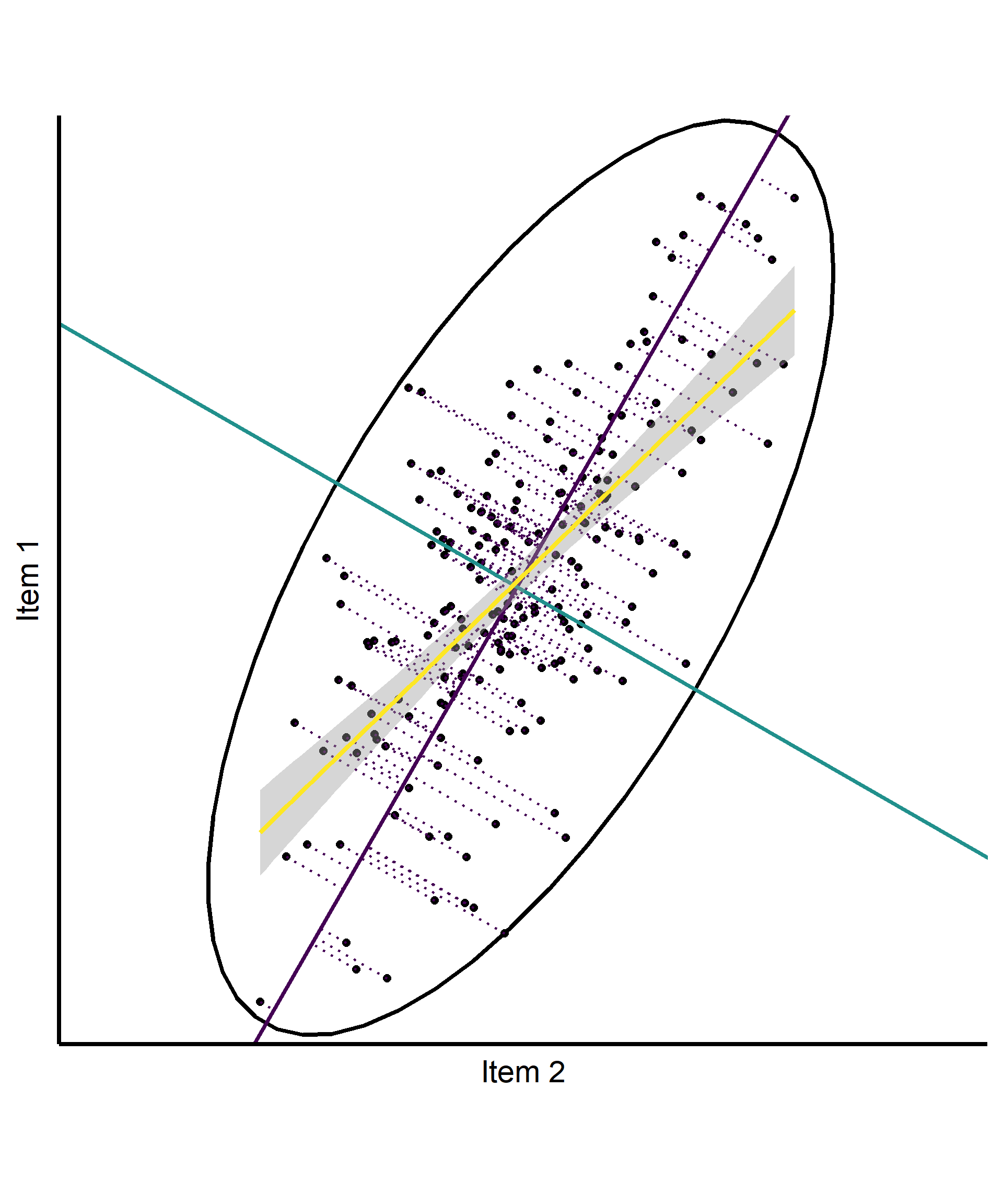
Basic intuition in 2d (based on PCA)
- 2 correlated Items
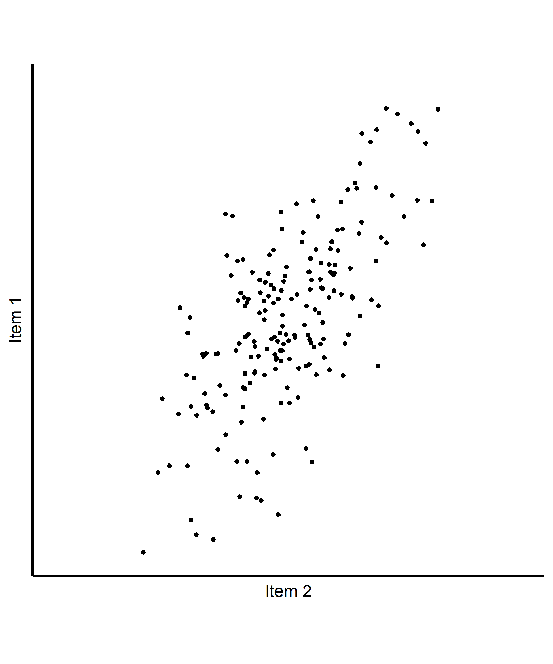
Basic intuition in 2d (based on PCA)
- 2 correlated Items
- Ellipse encapsulating the data based on \(cov(x, y)\)
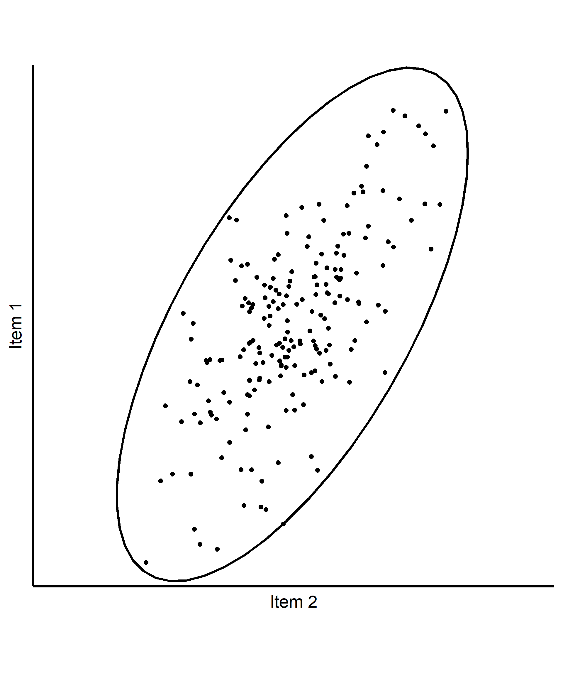
Basic intuition in 2d (based on PCA)
- 2 correlated Items
- Ellipse encapsulating the data based on \(cov(x, y)\)
- Find the axis along which the most variation occurs
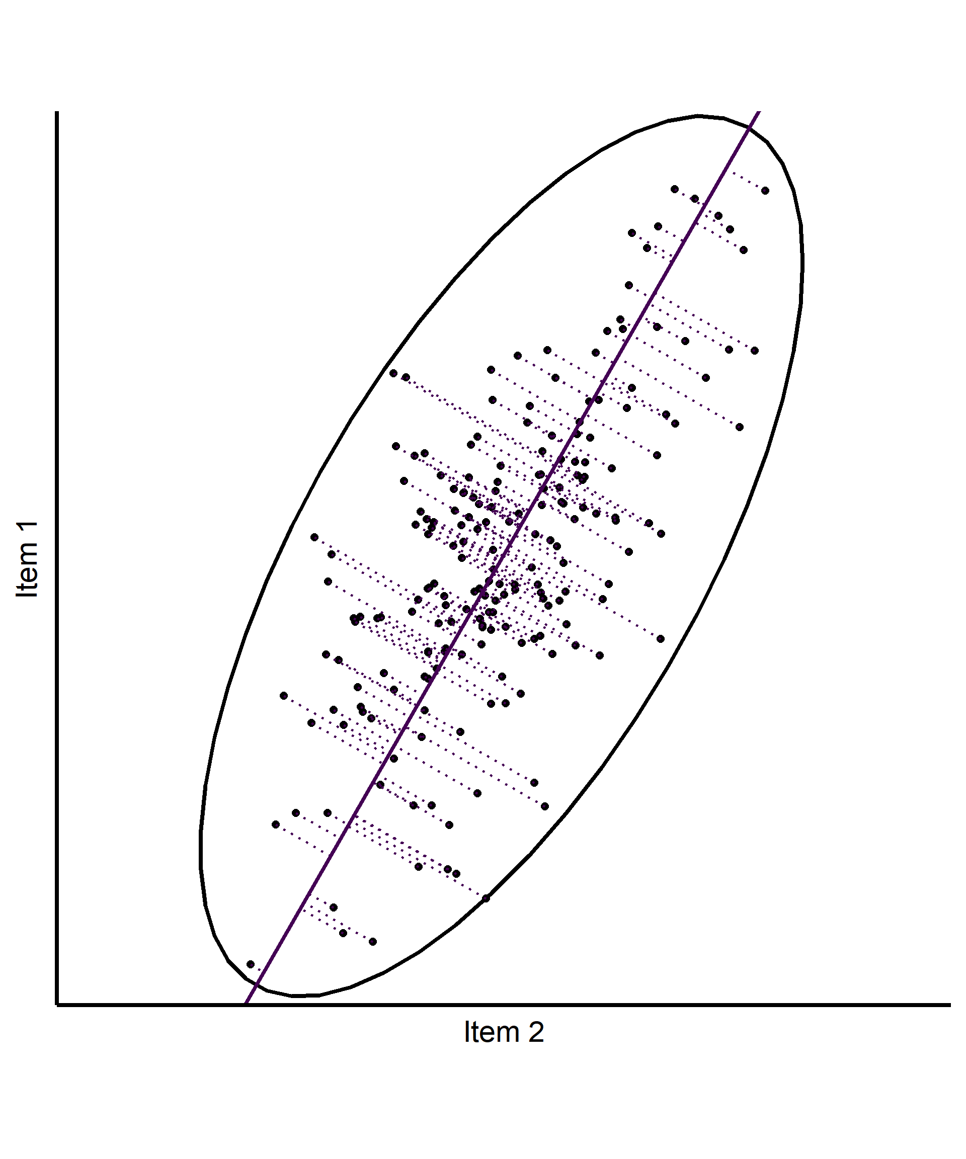
Basic intuition in 2d (based on PCA)
- 2 correlated Items
- Ellipse encapsulating the data based on \(cov(x, y)\)
- Find the axis along which the most variation occurs
- Find the axis along which the most residual variation occurs
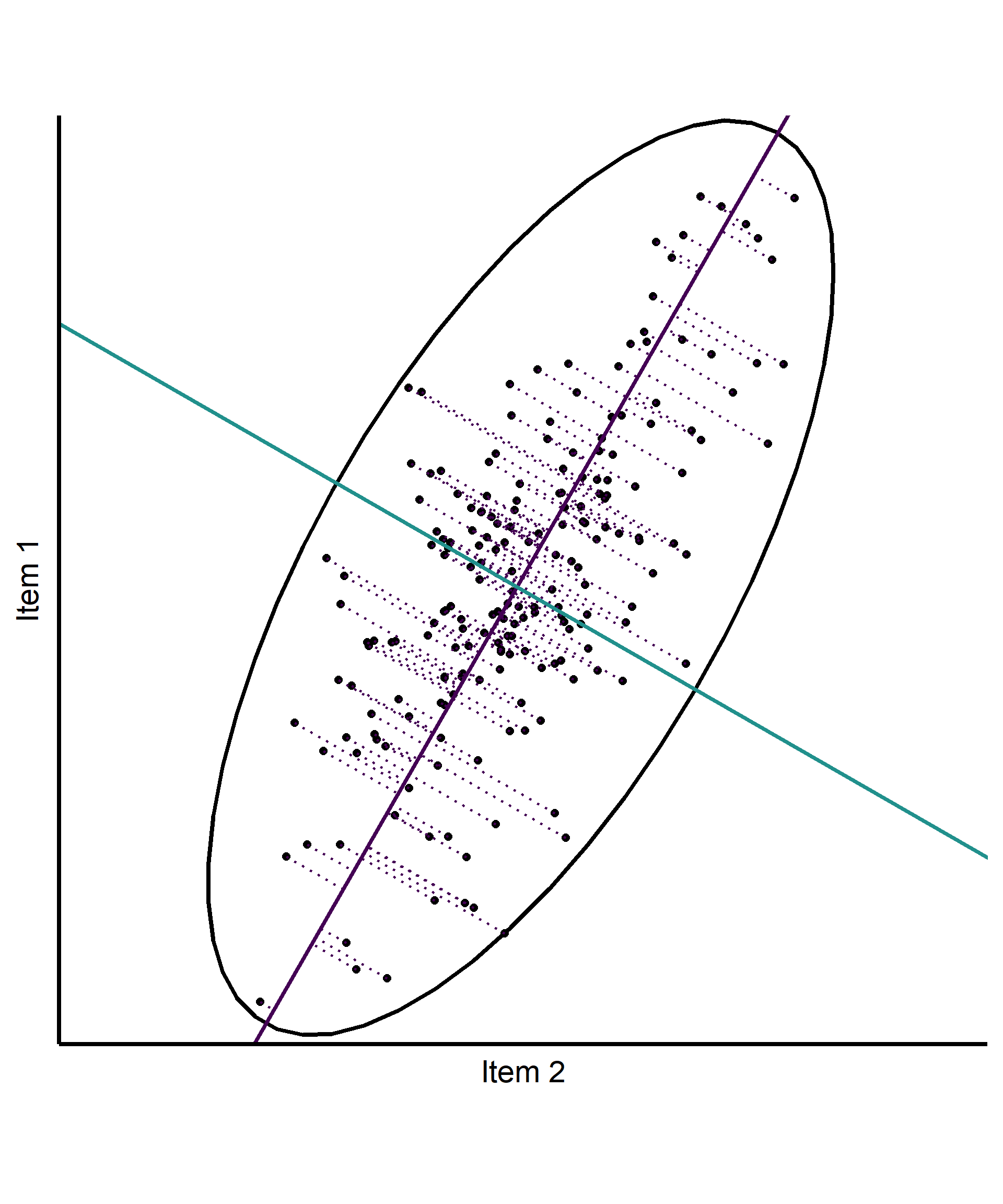
Basic intuition in 2d (based on PCA)
- 2 correlated Items
- Ellipse encapsulating the data based on \(cov(x, y)\)
- Find the axis along which the most variation occurs
- Find the axis along which the most residual variation occurs
- Note: These axes are different from the regression line
EFA vs. PCA
The first step: Decide between the common factor model and the principal components model
EFA:
- Based on common factor model.
- Account for the structure of correlations.
- Partition variance into common and unique factors.
- Assumes presence of measurement error.
PCA:
- Extract principle components out of MVs, that account for as much variance as possible.
- Create composite scores rather than latent variables.
- No distriction beween common and unique variances.
- Assumes error-free measurement of variables.
\(\rightarrow\) In most cases in psychological science, EFA is more appropriate than PCA, however, PCA is still often used (Fabrigar et al., 1999; Goretzko et al., 2021).
Steps of an EFA
- Calculate the correlation matrix \(R\).
- Test if \(R\) is suitable for EFA.
- Determine number of major common factors.
- Extract common factors.
- Rotate factors to obtain simple structure.
- Evaluate and interpret the model.
Test Suitability for EFA
If major CFs are present, correlations between MVs should be substantial.
- Bartletts test:
Test, if \(R\) is significantly different from \(I\).
ℹ 'x' was not a correlation matrix. Correlations are found from entered raw data.
✔ The Bartlett's test of sphericity was significant at an alpha level of .05.
  These data are probably suitable for factor analysis.

  𝜒²(28) = 5054.06, p < .001
R was not square, finding R from data$chisq
[1] 5054.06
$p.value
[1] 0
$df
[1] 28Test Suitability for EFA
If major CFs are present, correlations between MVs should be substantial.
- Bartletts test
- Kaiser-Meyer-Olkin (KMO) criterion:
\[ KMO=\frac{\sum\sum_{k\neq j}r^2_{jk}}{\sum\sum_{k\neq j}r^2_{jk} + \sum\sum_{k\neq j}p^2_{jk}} \]
\(\rightarrow\) Values should exceed .70 (Watkins, 2018) or .80 (Fabrigar & Wegener, 2012).
ℹ 'x' was not a correlation matrix. Correlations are found from entered raw data.
── Kaiser-Meyer-Olkin criterion (KMO) ──────────────────────────────────────────

✔ The overall KMO value for your data is marvellous.
  These data are probably suitable for factor analysis.

  Overall: 0.955

  For each variable:
      fun   friends     enjoy      hurt      part  commonly   chances attracted
    0.955     0.950     0.947     0.968     0.955     0.958     0.961     0.950
Kaiser-Meyer-Olkin factor adequacy
Call: psych::KMO(r = GRiPS_raw)
Overall MSA =  0.96
MSA for each item =
      fun   friends     enjoy      hurt      part  commonly   chances attracted
     0.96      0.95      0.95      0.97      0.96      0.96      0.96      0.95
Factor Retention Criteria
How many CFs underly the MVs? Many criteria exist (for overviews, see, e.g., Auerswald & Moshagen, 2019; Goretzko, 2025)
- Kaiser-Guttman Criterion:
Compute the eigenvalues of \(R\), take the number of eigenvalues >1. Often used, but don’t use it!
ℹ 'x' was not a correlation matrix. Correlations are found from entered raw data.
Eigenvalues were found using SMC.

── Number of factors suggested by Kaiser-Guttmann criterion ────────────────────

◌ With SMC-determined eigenvalues:  1
Factor Retention Criteria
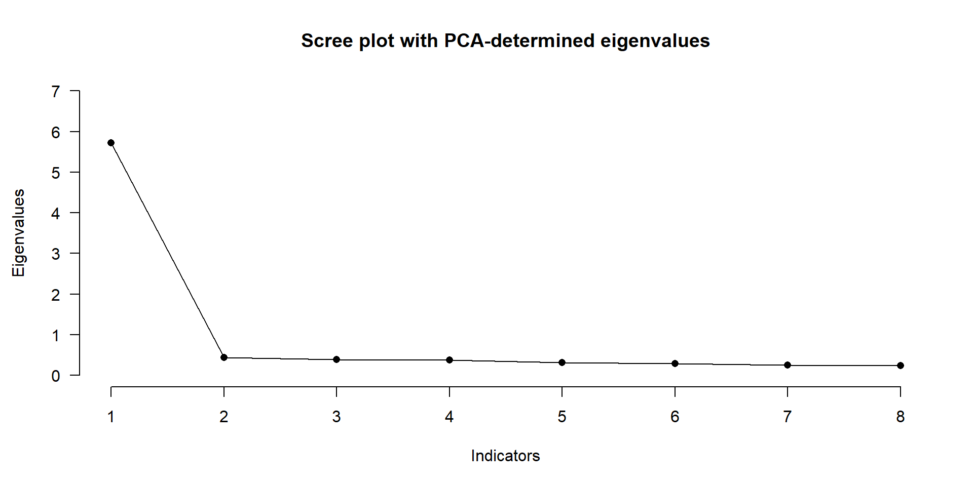
Factor Retention Criteria
- Kaiser-Guttman Criterion
- Scree-Plot
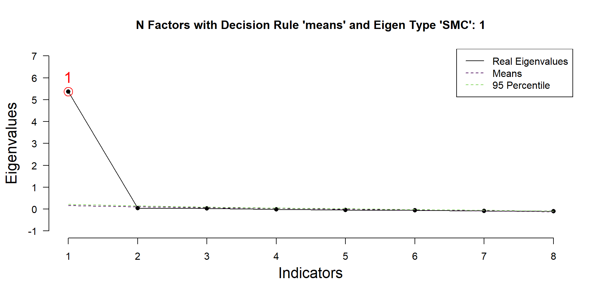
- Parallel analysis:
Compare the eigenvalues of \(R\) to average eigenvalues generated from \(b\) random Datasets of same \(N\) as \(R\).
Parallel Analysis performed using 1000 simulated random data sets
Eigenvalues were found using SMC

Decision rule used: means

── Number of factors to retain according to ────────────────────────────────────

◌ SMC-determined eigenvalues:  1
Factor Retention Criteria
- Kaiser-Guttman Criterion
- Scree-Plot
- Parallel analysis
- Many others, e.g. EKC (Braeken & van Assen, 2017), Hull-method (Lorenzo-Seva et al., 2011), Comparison data (Ruscio & Roche, 2012), NEST (Caron, 2025)
Good practice (see Auerswald & Moshagen, 2019): Use multiple criteria, e.g. parallel analysis and comparison data (Goretzko et al., 2021).
EFAtools::N_FACTORS(GRiPS_raw, show_progress = FALSE,
                    criteria = c("CD", "EKC", "HULL", "PARALLEL","SMT"))
── Tests for the suitability of the data for factor analysis ───────────────────

Bartlett's test of sphericity

✔ The Bartlett's test of sphericity was significant at an alpha level of .05.
  These data are probably suitable for factor analysis.

  𝜒²(28) = 5054.06, p < .001

Kaiser-Meyer-Olkin criterion (KMO)

✔ The overall KMO value for your data is marvellous with 0.955.
  These data are probably suitable for factor analysis.

── Number of factors suggested by the different factor retention criteria ──────

◌ Comparison data: 1
◌ Empirical Kaiser criterion: 1
◌ Hull method with CAF: 1
◌ Hull method with CFI: NA
◌ Hull method with RMSEA: NA
◌ Parallel analysis with PCA: 1
◌ Parallel analysis with SMC: 1
◌ Parallel analysis with EFA: 1
◌ Sequential 𝜒² model tests: 3
◌ Lower bound of RMSEA 90% confidence interval: 1
◌ Akaike Information Criterion: 3
Exercises
Factor Extraction
Multiple methods exist. ML and PAF are most popular (e.g., Watkins, 2018):
- PAF
- Non-parametric
- More robust
- ML:
- Assumes multivariate normality
- Less robust
- Can provide fit indices and standard errors
Extract Common Factors – PAF
\[P=\Lambda\Lambda^T+\Theta_\delta, \text{(no }\Phi \text{ as factors are orthogonal)} \]
\[\Downarrow \text{ use } R \text{ as approx. for }P\]
\[R=\Lambda\Lambda^T+\Theta_\delta\]
\[R-\Theta_\delta=\Lambda\Lambda^T\]
\[\Downarrow \text{ use } 1-\textit{SMC} \text{ as approx. for }\Theta_\delta \text{, i.e., } \textit{SMC} \text{ as approx. for } h^2\]
\[R-(1-SMC)=R_r=\Lambda\Lambda^T, \text{ with }R_r \text{ being the } \textit{reduced correlation matrix.}\]
\[\Rightarrow \text{Iteratively obtain } \Lambda \text{ using eigendecomposition of } R_r \text{ until } h^2 \text{ is stable.}\]
Extract Common Factors – ML
When using maximum likelihood (ML) estimation, parameters are found by minimizing
\[F_{ML}=ln|S| - ln|\Sigma| + trace(S\Sigma^{-1})-p\]
- \(S\): Sample covariance (in EFA, usually correlation) matrix
- \(\Sigma\): Model-implied covariance matrix
- p: Number of MVs
\(\rightarrow\) Perfect fitting model, \(S\) and \(\Sigma\) are identical, so \(F_{ML}\) is 0, as \(S\Sigma^{-1}=I\) and thus \(trace(S\Sigma^{-1})=p\).
Model Fit - \(\chi^2\)
- \(F_{ML}(N-1)\) is approx. \(\chi^2\)-distributed.
- \(\rightarrow\) Significance test, whether discrepancy between \(S\) and \(\Sigma\) is negligible.
- Problems:
- Unreasonable premise
- Needs large enough sample and normal data
- Inflated with very large samples, i.e., oversensitive.
- \(\rightarrow\) Therefore, additional fit indices are considered
Model Fit - Indices
Absolute fit indices, e.g.:
- RMSEA (\(\leq\).05, Hu & Bentler, 1999; but dependent on \(N\), \(df\), and model-specification Chen et al., 2008; Kenny et al., 2015)
- SRMR (\(\leq\).08, Hu & Bentler, 1999)
Incremental fit indices, e.g. (reduction in misfit compared to baseline, usually zero covariances):
- TLI (\(\geq\).95, Hu & Bentler, 1999)
- CFI (\(\geq\).95, Hu & Bentler, 1999)
\(\rightarrow\) Report multiple indices (Chen et al., 2008; Hu & Bentler, 1999; Moshagen & Auerswald, 2018).
\(\rightarrow\) Don’t overrely on cut-off values (Chen et al., 2008; Kenny et al., 2015; Lai & Green, 2016).
\(\rightarrow\) RMSEA and TLI good measures of fit and fitting propensity according to (Bader & Moshagen, 2025), but see also (Bonifay et al., 2025).
Exercises
Factor Rotation - Basics
- Unrotated solutions are hard to interpret
- Rotation strives for simple structure:
- Each CF has large loadings for some MVs and small loadings for other MVs.
- Subset of MVs defining CFs should not substantially overlap.
- Each MV should be influenced by only a subset of CFs.
- \(\rightarrow\) Cross-loadings can be ok.
- Two kinds of rotation:
- Orthogonal: Uncorrelated CFs (e.g., Varimax)
- Oblique: Correlated CFs (e.g., Promax, Oblimin) \(\rightarrow\) Preferred!
Factor Rotation - Graphical Intuition
Factor Rotation - Costs of Oblique Rotation
Interpretation of factor loadings differs between orthogonal and oblique rotations:
- Orthogonal rotation: Correlation between CFs and MVs, thus \(R^2=h^2=\lambda^2\).
- Oblique rotation: Two types of loadings
- Structure coefficients (\(\Lambda\Phi\)): Correlation between CFs and MVs, thus \(R^2=\lambda^2\).
- Pattern coefficients (\(\Lambda\): Like standardized, partial regression coeffs: Correlation between CFs and MVs after controlling for the influence of all other CFs. \(\rightarrow\) Can exceed \(|1.00|\).
Exercises
Interpretation
- Goodness of Fit?
- Simple structure present?
- Directions and size of pattern coefficients and factor correlations reasonable?
- Size of communalities (below .4 is low, .4 to .7 is good, .7 or higher is ideal)?
- Heywood cases present (communalities/structure coefficients > 1)?
- Proportion of variance explained?
Interpretation
- Goodness of Fit?
- Simple structure present?
- Directions and size of pattern coefficients and factor correlations reasonable?
- Size of communalities \(h^2\) (below .4 is low, .4 to .7 is good, .7 or higher is ideal)?
- Heywood cases present (communalities/structure coefficients > 1)?
- Proportion of variance explained?
- Large difference between \(R\) and Model-implied \(R\) (\(R_M=\Lambda\Phi\Lambda^T+\Theta_\delta\))?
\(\rightarrow\) Run in R
### Differences between R and R_model:

# EFAtools
fit <- EFAtools::EFA(temp, n_factors = 2,
                     rotation = "promax")
round(R - fit$model_implied_R, 2)

# psych
fit <- psych::fa(temp, nfactors = 2)
Lambda <- fit$loadings
Phi <- fit$Phi
Theta <- diag(fit$uniquenesses)
R_model <- Lambda %*% Phi %*% t(Lambda) + Theta
round(R - R_model, 2)

# lavaan more complicated -> see solutions in exercises
Exercises
Section F - Evaluation and Interpretation in the EFA exercises
Categorical or skewed data
- Skewed / non-normal: Use ML (or WLS) with polychoric correlations (Goretzko et al., 2021) or robust ML.
- With categorical data, use DWLS-estimation and polychoric correlation
- Note: Fit indices may be biased (e.g., Savalei, 2021; Shi & Maydeu-Olivares, 2020; Xia & Yang, 2019) ->
{lavaan}can provide adjusted versions.
# psych option (only WLS, not DWLS):
psych::fa(temp, nfactors = 2, fm = "wls",
          cor = "poly", rotate = "oblimin")

### lavaan options
# robust ML with scaled
lavaan::efa(data = temp, nfactors = 2, rotation = "oblimin",
            estimator = "MLR")
# polychorric cors with DWLS estimation
lavaan::efa(data = temp, nfactors = 2, rotation = "oblimin",
            ordered = TRUE, estimator = "WLSM")
Exercises
Recommendations (Goretzko et al., 2021)
- Use 4-5 MVs per factor
- Sample size: at least 300, better 400
- Use polychoric correlations with categorical and non-normal/skewed response data
- Use multiple factor retention criteria
- Use ML-estimation when data allows, otherwise use, e.g., PAF or WLS
- Use oblique rotations
Reporting an EFA (see Watkins, 2018)
- MVs
- Sample size
- Data characteristics
- Software and version
- Appropriateness of data for EFA
- Correlation method
- Factor retention methods and # factors
- Factor model (EFA/PCA)
- Estimation method (ML, PAF, etc.)
- Factor rotation method
- % variance explained by factors (spec. before or after rotation)
- Complete pattern matrix
- Interfactor correlations
- Reliability of factors
- Structure matrix (if different from pattern matrix)
- Eigenvalues for all factors
- Correlation matrix
References
Auerswald, M., & Moshagen, M. (2019). How to determine the number of factors to retain in exploratory factor analysis: A comparison of extraction methods under realistic conditions. Psychological Methods, 24(4), 468–491. https://doi.org/10.1037/met0000200
Bader, M., & Moshagen, M. (2025). Assessing the fitting propensity of factor models. Psychological Methods, 30(2), 254–270. https://doi.org/10.1037/met0000529
Bonifay, W., Cai, L., Falk, C. F., & Preacher, K. J. (2025). Reassessing the fitting propensity of factor models. Psychological Methods. https://doi.org/10.1037/met0000735
Braeken, J., & van Assen, M. A. (2017). An empirical Kaiser criterion. Psychological Methods, 22, 450–466. https://doi.org/10.1037/ met0000074
Caron, P.-O. (2025). A Comparison of the Next Eigenvalue Sufficiency Test to Other Stopping Rules for the Number of Factors in Factor Analysis. Educational and Psychological Measurement, 00131644241308528. https://doi.org/10.1177/00131644241308528
Chen, F., Curran, P. J., Bollen, K. A., Kirby, J., & Paxton, P. (2008). An Empirical Evaluation of the Use of Fixed Cutoff Points in RMSEA Test Statistic in Structural Equation Models. Sociological Methods & Research, 36(4), 462–494. https://doi.org/10.1177/0049124108314720
Fabrigar, L. R., & Wegener, D. T. (2012). Exploratory Factor Analysis. Oxford University Press.
Fabrigar, L. R., Wegener, D. T., MacCallum, R. C., & Strahan, E. J. (1999). Evaluating the Use of Exploratory Factor Analysis in Psychological Research. Psychological Methods, 4(3), 272–299.
Goretzko, D. (2025). How many factors to retain in exploratory factor analysis? A critical overview of factor retention methods. Psychological Methods. https://doi.org/10.1037/met0000733
Goretzko, D., Pham, T. T. H., & Bühner, M. (2021). Exploratory factor analysis: Current use, methodological developments and recommendations for good practice. Current Psychology, 40(7), 3510–3521. https://doi.org/10.1007/s12144-019-00300-2
Hu, L., & Bentler, P. M. (1999). Cutoff criteria for fit indexes in covariance structure analysis: Conventional criteria versus new alternatives. Structural Equation Modeling: A Multidisciplinary Journal, 6(1), 1–55. https://doi.org/10.1080/10705519909540118
Kenny, D. A., Kaniskan, B., & McCoach, D. B. (2015). The Performance of RMSEA in Models With Small Degrees of Freedom. Sociological Methods & Research, 44(3), 486–507. https://doi.org/10.1177/0049124114543236
Lai, K., & Green, S. B. (2016). The Problem with Having Two Watches: Assessment of Fit When RMSEA and CFI Disagree. Multivariate Behavioral Research, 51(2-3), 220–239. https://doi.org/10.1080/00273171.2015.1134306
Lorenzo-Seva, U., Timmerman, M. E., & Kiers, H. A. (2011). The Hull method for selecting the number of common factors. Multivariate Behavioral Research, 46(2), 340–364.
Moshagen, M., & Auerswald, M. (2018). On congruence and incongruence of measures of fit in structural equation modeling. Psychological Methods, 23(2), 318–336. https://doi.org/10.1037/met0000122
Ruscio, J., & Roche, B. (2012). Determining the number of factors to retain in an exploratory factor analysis using comparison data of known factorial structure. Psychological Assessment, 24, 282–292. https://doi.org/10.1037/a0025697
Savalei, V. (2021). Improving Fit Indices in Structural Equation Modeling with Categorical Data. Multivariate Behavioral Research, 56(3), 390–407. https://doi.org/10.1080/00273171.2020.1717922
Shi, D., & Maydeu-Olivares, A. (2020). The Effect of Estimation Methods on SEM Fit Indices. Educational and Psychological Measurement, 80(3), 421–445. https://doi.org/10.1177/0013164419885164
Steiner, M. D., & Frey, R. (2021). Representative design in psychological assessment: A case study using the Balloon Analogue Risk Task (BART). Journal of Experimental Psychology: General, 150(10), 2117–2136. https://doi.org/10.1037/xge0001036
Watkins, M. W. (2018). Exploratory Factor Analysis: A Guide to Best Practice. Journal of Black Psychology, 44(3), 219–246. https://doi.org/10.1177/0095798418771807
Xia, Y., & Yang, Y. (2019). RMSEA, CFI, and TLI in structural equation modeling with ordered categorical data: The story they tell depends on the estimation methods. Behavior Research Methods, 51(1), 409–428. https://doi.org/10.3758/s13428-018-1055-2
Zhang, D. C., Highhouse, S., & Nye, C. D. (2019). Development and validation of the General Risk Propensity Scale (GRiPS). Journal of Behavioral Decision Making, 32(2), 152–167. https://doi.org/10.1002/bdm.2102
![]()
Introduction to Factor Analysis - GSP 2025