Workshop: Introduction to Factor Analysis - GSP 2025
Author
Affiliation
Markus Steiner
Institute for Mental and Organisational Health, FHNW
Published
05 June, 2025
A – Setup
Exercise A1. Open the Intro2FactorAnalysis RStudio-Project and create a new R-script EFA_exercises.R.
Exercise A2. Load the lavaan, psych, EFAtools and tidyverse packages (tidyverse is for data-wrangling; but feel free to use any style of data-wrangling).
Show Solution
library(lavaan)
This is lavaan 0.6-19
lavaan is FREE software! Please report any bugs.
library(psych)
Attache Paket: 'psych'
Das folgende Objekt ist maskiert 'package:lavaan':

    cor2cov
library(EFAtools)
Attache Paket: 'EFAtools'
Das folgende Objekt ist maskiert 'package:psych':

    KMO
── Conflicts ────────────────────────────────────────── tidyverse_conflicts() ──
✖ggplot2::%+%() masks psych::%+%()
✖ggplot2::alpha() masks psych::alpha()
✖dplyr::filter() masks stats::filter()
✖dplyr::lag() masks stats::lag()
ℹ Use the conflicted package (<http://conflicted.r-lib.org/>) to force all conflicts to become errors
B – Suitability for factor analysis
Exercise B1. The 01_data folder contains two datasets. Load the gad7.csv dataset using the code below. It contains responses from over 13’000 participants to multiple scales, including the seven items of the generalized anxiety disorder (GAD-7) scale (e.g., Kroenke et al., 2007), that were collected alongside with other scales by Sauter and Draschkow, 2017 (the complete dataset is openly available at osf.io).
gad7 <-read_csv("01_data/gad7.csv") %>%select(GAD1:GAD7) # only keep GAD-items for this exerciseglimpse(gad7)
The questionnaire asks subjects, How often have you been bothered by the following over the past 2 weeks? and then presents the follwing items with a scale from 0 (not at all) to 3 (nearly every day):
Feeling nervous, anxious or on edge.
Not being able to stop or control worrying.
Worrying too much about different things.
Trouble relaxing.
Being so restless that it’s hard to sit still.
Becoming easily annoyed or irritable.
Feeling afraid as if something awful might hapen.
It’s a screening tool generalized anxiety disorder, but has been found to also be an acceptable screening for panic disorder, social anxiety, and PTSD (see, e.g., Plummer et al., 2016).
Exercise B2. Look at the correlation matrix of the gad7 (Hint: use cor()). Do you think the data are suitable for factor analysis?
The correlations are heterogenous and moderate to large in size. This matrix clearly is very different from an identity matrix and is thus probably suitable for factor analysis.
Exercise B3. Using BARTLETT() and KMO() of {EFAtools}, test whether the gad7 is suitable for factor analysis (Note:KMO() exists also in the {psych} package, so use EFAtools::KMO() to explicitly use the EFAtools version). Interpret the output
Show Solution
BARTLETT(gad7)
ℹ 'x' was not a correlation matrix. Correlations are found from entered raw data.
✔ The Bartlett's test of sphericity was significant at an alpha level of .05.
  These data are probably suitable for factor analysis.

  𝜒²(21) = 38687, p < .001
EFAtools::KMO(gad7)
ℹ 'x' was not a correlation matrix. Correlations are found from entered raw data.
──Kaiser-Meyer-Olkin criterion (KMO)──────────────────────────────────────────✔ The overall KMO value for your data is meritorious.
These data are probably suitable for factor analysis.
Overall:0.891For each variable:
GAD1 GAD2 GAD3 GAD4 GAD5 GAD6 GAD7
0.896 0.843 0.876 0.911 0.902 0.924 0.928
Both tests clearly indicate that the data are suitable for factor analysis. The correlation matrix is significantly different from an identity matrix (Bartlett’s test) and when the variance of the remaining items is partialed out from any of the GAD items, only a small proportion of the variance remains (KMO).
Exercise B4. Now use the {psych} versions of the test (cortest.bartlett() and psych::KMO()). Do the results match the previous exercise? In practice, use whichever version you like.
The results match, both packages provide the same statistics.
C – Factor retention
Exercise C1. One of the most important questions in the process of an EFA is how many factors to retain. In many published studies, you will see the Kaiser-Guttman (also often called eigenvalue-greater-one) criterion or the Scree-test being used to this end. You should, however, not use these criteria, as they don’t perform well. Instead, use and compare multiple criteria (see Auerswald & Moshagen, 2019), e.g., parallel analysis and comparison data (Goretzko et al., 2021). Using N_FACTORS() from {EFAtools}, compute and compare different criteria. Do they mostly agree or disagree?
Show Solution
set.seed(42) # ensure same results with multiple runsN_FACTORS(gad7, criteria =c("CD", "EKC", "HULL", "PARALLEL","SMT"),method ="ML")
──Tests for the suitability of the data for factor analysis───────────────────Bartlett's test of sphericity✔ The Bartlett's test of sphericity was significant at an alpha level of .05.
These data are probably suitable for factor analysis.
𝜒²(21) = 38687, p < .001
Kaiser-Meyer-Olkin criterion (KMO)✔ The overall KMO value for your data is meritorious with 0.891.
These data are probably suitable for factor analysis.
──Number of factors suggested by the different factor retention criteria──────◌ Comparison data: 2◌ Empirical Kaiser criterion: 1◌ Hull method with CAF: 2◌ Hull method with CFI: 1◌ Hull method with RMSEA: 2◌ Parallel analysis with PCA: 1◌ Parallel analysis with SMC: 2◌ Parallel analysis with EFA: 3◌ Sequential 𝜒² model tests: NA◌ Lower bound of RMSEA 90% confidence interval: 2◌ Akaike Information Criterion: 3
This is a difficult situation: Following Goretzko et al. (2021) and looking at parallel analysis and comparison data, there is already some disagreement. Fabrigar & Wegener (2012) argue that in the case of EFA, parallel analysis based on the reduced correlation matrix (i.e, with SMC or with EFA in the output above) is the most sensible approach, however Auerswald & Moshagen (2019) discuss simulation studies on this topic that seem to favor parallel analysis with the unreduced correlation matrx (i.e., with PCA in the output above). So what now? We can test multiple solutions (e.g., 1 and 2 factors) and compare them on global an local fit. Moreover, it makes sense to look at the items (see above) and think about substantive reasons for different number of factors (although domain-specific expertise is needed here, which I don’t have…).
Exercise C2. Use the {psych} package to determine the number of factors (e.g., nfactors() and fa.parallel()).
Show Solution
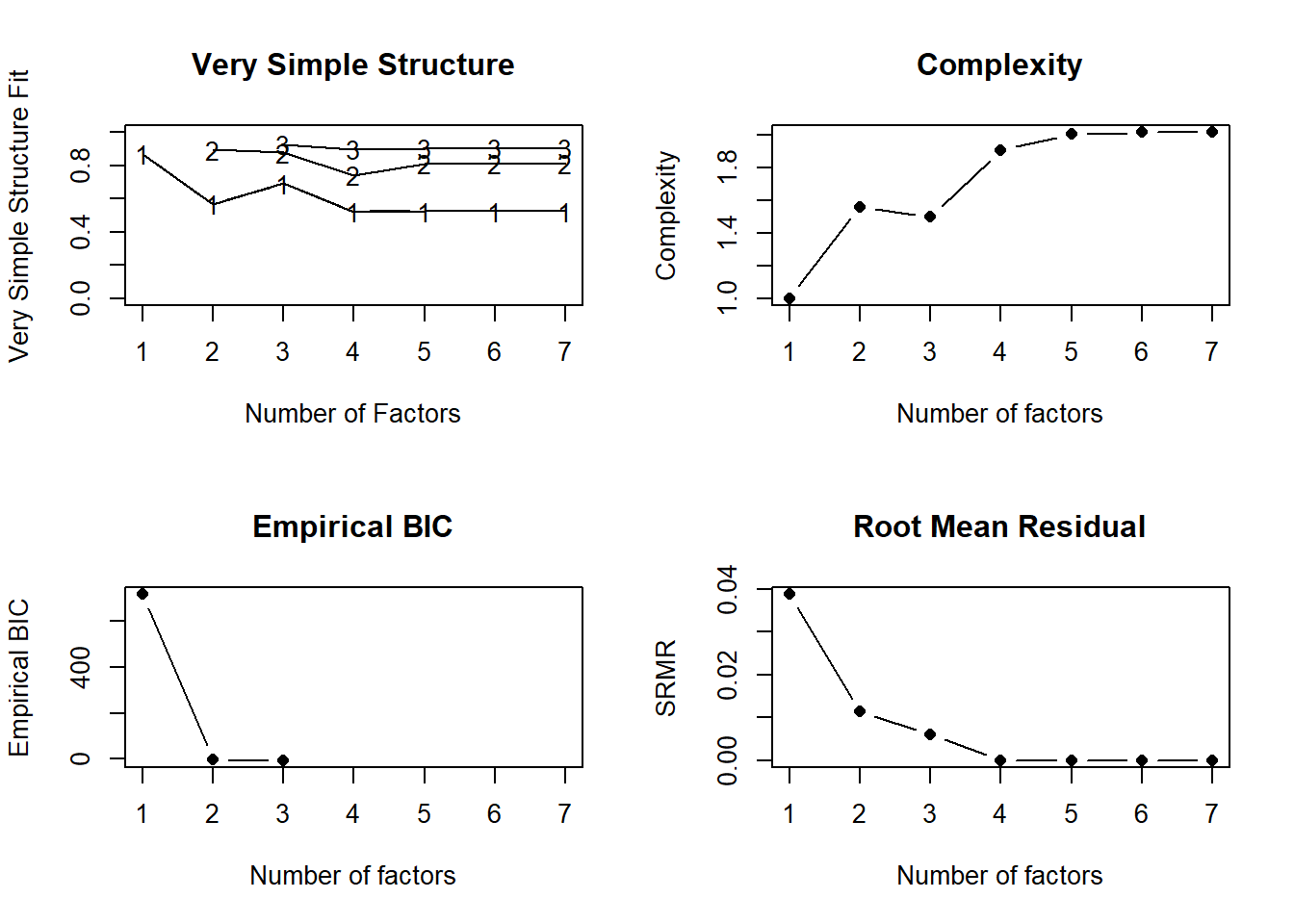
nfactors(gad7)
Number of factors
Call: vss(x = x, n = n, rotate = rotate, diagonal = diagonal, fm = fm,
    n.obs = n.obs, plot = FALSE, title = title, use = use, cor = cor)
VSS complexity 1 achieves a maximimum of 0.87  with  1  factors
VSS complexity 2 achieves a maximimum of 0.89  with  2  factors
The Velicer MAP achieves a minimum of 0.04  with  1  factors
Empirical BIC achieves a minimum of  -7.36  with  3  factors
Sample Size adjusted BIC achieves a minimum of  55.02  with  3  factors

Statistics by number of factors
  vss1 vss2   map dof   chisq     prob sqresid  fit RMSEA  BIC SABIC complex
1 0.87 0.00 0.038  14 1.4e+03 3.3e-292     2.2 0.87 0.086 1275  1319     1.0
2 0.57 0.89 0.076   8 1.7e+02  1.3e-31     1.7 0.89 0.038   89   115     1.6
3 0.69 0.88 0.151   3 7.4e+01  5.9e-16     1.2 0.93 0.042   45    55     1.5
4 0.52 0.74 0.345  -1 6.2e-06       NA     1.5 0.91    NA   NA    NA     1.9
5 0.53 0.81 0.572  -4 2.0e-08       NA     1.5 0.91    NA   NA    NA     2.0
6 0.53 0.81 1.000  -6 1.2e-11       NA     1.5 0.91    NA   NA    NA     2.0
7 0.53 0.81    NA  -7 1.2e-11       NA     1.5 0.91    NA   NA    NA     2.0
   eChisq    SRMR eCRMS  eBIC
1 8.5e+02 3.9e-02 0.048 717.9
2 7.3e+01 1.1e-02 0.018  -3.2
3 2.1e+01 6.1e-03 0.016  -7.4
4 2.8e-06 2.2e-06    NA    NA
5 8.0e-09 1.2e-07    NA    NA
6 2.5e-12 2.1e-09    NA    NA
7 2.5e-12 2.1e-09    NA    NA
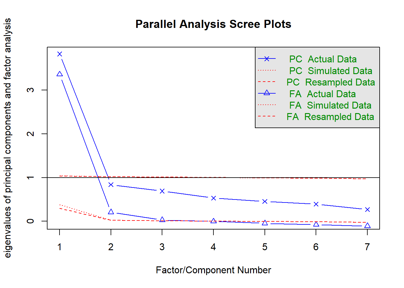
fa.parallel(gad7)
Parallel analysis suggests that the number of factors = 3 and the number of components = 1
{psych} also suggests between 1 and 3 factors, though with some additional factor retention criteria, e.g., the Very Simple Structure criterion (VSS) and Minimum Average Parcels criterion (MAP).
D – Factor extraction
Exercise D1. The next step is to extract the desired number of factors. Let’s start with a 1-factor solution. Here, no rotation is necessary/possible, as we only extract a single latent dimension. Using EFA() from {EFAtools}, extract one factor with principal axis factoring (PAF), the default option. Save the output as gad_1f. How does the solution look like?
Show Solution
gad_1f <-EFA(gad7, n_factors =1)
ℹ 'x' was not a correlation matrix. Correlations are found from entered raw data.
gad_1f
EFA performed with type = 'EFAtools', method = 'PAF', and rotation = 'none'.
──Unrotated Loadings────────────────────────────────────────────────────────── F1 h2 u2 GAD1 .770 .593 .407
GAD2 .834 .695 .305
GAD3 .786 .618 .382
GAD4 .717 .515 .485
GAD5 .474 .224 .776
GAD6 .499 .249 .751
GAD7 .678 .460 .540
──Variances Accounted for───────────────────────────────────────────────────── F1 SS loadings 3.355
Prop Tot Var 0.479
──Model Fit───────────────────────────────────────────────────────────────────CAF: .45
df: 14
Most loadings are relatively high, but GAD5 and GAD6 have lower loadings. These are the items Being so restless that it’s hard to sit still and Becoming easily annoyed or irritable. Communalities are substantial (around .6) for items 1 to 4, except for Items 5-7.
Exercise D2. PAF is a non-parametric procedure and as such cannot provide often-used fit indices. Rerun the model, but this time, add the argument method = "ML" to use maximum-likelihood estimation. Do the two solutions agree?
Show Solution
gad_1f_ml <-EFA(gad7, n_factors =1, method ="ML")
ℹ 'x' was not a correlation matrix. Correlations are found from entered raw data.
gad_1f_ml
EFA performed with type = 'EFAtools', method = 'ML', and rotation = 'none'.
──Unrotated Loadings────────────────────────────────────────────────────────── F1 h2 u2 GAD1 .776 .602 .398
GAD2 .853 .728 .272
GAD3 .802 .643 .357
GAD4 .697 .486 .514
GAD5 .451 .203 .797
GAD6 .477 .228 .772
GAD7 .674 .454 .546
──Variances Accounted for───────────────────────────────────────────────────── F1 SS loadings 3.343
Prop Tot Var 0.478
──Model Fit───────────────────────────────────────────────────────────────────𝜒²(14) = 1314.65, p < .001
CFI = .98
RMSEA [90% CI] = .08 [.08; .09]
AIC = 1286.65
BIC = 1181.54
CAF = .45
The solutions differ slightly, but agree in general. In addition, we see that the fit indices indicate acceptable to good fit. But more on these indices in the CFA-session!
Exercise D3. Rerun the model using fa() from {psych} (see the help page for details: ?fa. Compare to the outputs above. Do they agree in general?
Show Solution
gad_1f_psych <-fa(gad7, nfactors =1)gad_1f_psych
Factor Analysis using method =  minres
Call: fa(r = gad7, nfactors = 1)
Standardized loadings (pattern matrix) based upon correlation matrix
      MR1   h2   u2 com
GAD1 0.77 0.59 0.41   1
GAD2 0.83 0.70 0.30   1
GAD3 0.79 0.62 0.38   1
GAD4 0.72 0.51 0.49   1
GAD5 0.47 0.22 0.78   1
GAD6 0.50 0.25 0.75   1
GAD7 0.68 0.46 0.54   1

                MR1
SS loadings    3.36
Proportion Var 0.48

Mean item complexity =  1
Test of the hypothesis that 1 factor is sufficient.

df null model =  21  with the objective function =  2.87 with Chi Square =  38687
df of  the model are 14  and the objective function was  0.1

The root mean square of the residuals (RMSR) is  0.04
The df corrected root mean square of the residuals is  0.05

The harmonic n.obs is  13464 with the empirical chi square  851.04  with prob <  1.3e-172
The total n.obs was  13464  with Likelihood Chi Square =  1407.86  with prob <  3.3e-292

Tucker Lewis Index of factoring reliability =  0.946
RMSEA index =  0.086  and the 90 % confidence intervals are  0.082 0.09
BIC =  1274.75
Fit based upon off diagonal values = 0.99
Measures of factor score adequacy
                                                   MR1
Correlation of (regression) scores with factors   0.94
Multiple R square of scores with factors          0.89
Minimum correlation of possible factor scores     0.77
The results are very similar.
Exercise D4. Finally, use efa() from {lavaan} fit the model. Note that the print output is very minimalist, use summary() for a more extensive output.
This is lavaan 0.6-19 -- running exploratory factor analysis

  Estimator                                         ML
  Rotation method                       GEOMIN OBLIQUE
  Geomin epsilon                                 0.001
  Rotation algorithm (rstarts)                GPA (30)
  Standardized metric                             TRUE
  Row weights                                     None

  Number of observations                         13464

Fit measures:
                  aic      bic    sabic    chisq df pvalue   cfi rmsea
  nfactors = 1 213304 213409.1 213364.6 1314.744 14      0 0.966 0.083

Eigenvalues correlation matrix:

    ev1     ev2     ev3     ev4     ev5     ev6     ev7
  3.824   0.837   0.692   0.531   0.456   0.392   0.269

Standardized loadings: (* = significant at 1% level)

         f1       unique.var   communalities
GAD1  0.776*           0.398           0.602
GAD2  0.853*           0.272           0.728
GAD3  0.802*           0.357           0.643
GAD4  0.697*           0.514           0.486
GAD5  0.451*           0.797           0.203
GAD6  0.477*           0.772           0.228
GAD7  0.674*           0.546           0.454

                           f1
Sum of squared loadings 3.343
Proportion of total     1.000
Proportion var          0.478
Cumulative var          0.478
Again, results match more or less with the previous solutions.
Pick your software!
You’ve now tested three different packages. For the following exercises, choose the one you like most and work just work with that. I won’t add more exercises where you compare the three options. I will provide the solutions for all three packages for the future exercises.
As {lavaan} and {psych} provide the most features and have been continuously developed for years and both have a huge user-base, relying on one of them probably makes sense.
E – Factor rotation
Exercise E1. In the previous solution, we extracted one factor and thus didn’t need a rotation. Now, extract two factors and specify an orthogonal rotation (e.g., varimax). Save it as gad_2f_orth. Does the solution provide simple structure? How is the model fit?
Factor Analysis using method =  minres
Call: fa(r = gad7, nfactors = 2, rotate = "varimax")
Standardized loadings (pattern matrix) based upon correlation matrix
      MR1  MR2   h2   u2 com
GAD1 0.66 0.40 0.59 0.41 1.6
GAD2 0.84 0.30 0.79 0.21 1.2
GAD3 0.73 0.33 0.65 0.35 1.4
GAD4 0.48 0.57 0.55 0.45 1.9
GAD5 0.19 0.57 0.36 0.64 1.2
GAD6 0.28 0.47 0.30 0.70 1.6
GAD7 0.55 0.39 0.45 0.55 1.8

                       MR1  MR2
SS loadings           2.32 1.37
Proportion Var        0.33 0.20
Cumulative Var        0.33 0.53
Proportion Explained  0.63 0.37
Cumulative Proportion 0.63 1.00

Mean item complexity =  1.6
Test of the hypothesis that 2 factors are sufficient.

df null model =  21  with the objective function =  2.87 with Chi Square =  38687
df of  the model are 8  and the objective function was  0.01

The root mean square of the residuals (RMSR) is  0.01
The df corrected root mean square of the residuals is  0.02

The harmonic n.obs is  13464 with the empirical chi square  72.83  with prob <  1.3e-12
The total n.obs was  13464  with Likelihood Chi Square =  165.21  with prob <  1.3e-31

Tucker Lewis Index of factoring reliability =  0.989
RMSEA index =  0.038  and the 90 % confidence intervals are  0.033 0.043
BIC =  89.14
Fit based upon off diagonal values = 1
Measures of factor score adequacy
                                                   MR1  MR2
Correlation of (regression) scores with factors   0.88 0.72
Multiple R square of scores with factors          0.77 0.52
Minimum correlation of possible factor scores     0.54 0.04
Warning: lavaan->lav_model_vcov():
   The variance-covariance matrix of the estimated parameters (vcov) does not
   appear to be positive definite! The smallest eigenvalue (= -1.022153e-20)
   is smaller than zero. This may be a symptom that the model is not
   identified.
This is lavaan 0.6-19 -- running exploratory factor analysis

  Estimator                                         ML
  Rotation method                   VARIMAX ORTHOGONAL
  Rotation algorithm (rstarts)                GPA (30)
  Standardized metric                             TRUE
  Row weights                                   Kaiser

  Number of observations                         13464

Fit measures:
                    aic      bic    sabic   chisq df pvalue   cfi rmsea
  nfactors = 2 212158.9 212309.1 212245.5 157.704  8      0 0.996 0.037

Eigenvalues correlation matrix:

    ev1     ev2     ev3     ev4     ev5     ev6     ev7
  3.824   0.837   0.692   0.531   0.456   0.392   0.269

Standardized loadings: (* = significant at 1% level)

         f1      f2       unique.var   communalities
GAD1  0.657*  0.401*           0.408           0.592
GAD2  0.844*      .*           0.199           0.801
GAD3  0.720*  0.349*           0.360           0.640
GAD4  0.472*  0.575*           0.447           0.553
GAD5      .*  0.551*           0.656           0.344
GAD6      .*  0.486*           0.695           0.305
GAD7  0.541*  0.396*           0.551           0.449

                              f1    f2 total
Sum of sq (ortho) loadings 2.287 1.398 3.685
Proportion of total        0.621 0.379 1.000
Proportion var             0.327 0.200 0.526
Cumulative var             0.327 0.526 0.526
Most items load on both factors, i.e., there are multiple cross-loadings, thus there’s no real simple structure. The communalities are a bit higher than in the previous solution, global model fit is substantially better.
Exercise E2. Now rerun the previous analysis but use an oblique rotation (e.g., promax). Save it as gad_2f_oblq. Is the solution very different from the one based on the orthogonal rotation?
Factor Analysis using method =  minres
Call: fa(r = gad7, nfactors = 2, rotate = "promax")
Standardized loadings (pattern matrix) based upon correlation matrix
       MR1   MR2   h2   u2 com
GAD1  0.66  0.14 0.59 0.41 1.1
GAD2  0.97 -0.12 0.79 0.21 1.0
GAD3  0.81 -0.01 0.65 0.35 1.0
GAD4  0.30  0.49 0.55 0.45 1.7
GAD5 -0.09  0.67 0.36 0.64 1.0
GAD6  0.09  0.47 0.30 0.70 1.1
GAD7  0.51  0.20 0.45 0.55 1.3

                       MR1  MR2
SS loadings           2.56 1.13
Proportion Var        0.37 0.16
Cumulative Var        0.37 0.53
Proportion Explained  0.69 0.31
Cumulative Proportion 0.69 1.00

 With factor correlations of
     MR1  MR2
MR1 1.00 0.76
MR2 0.76 1.00

Mean item complexity =  1.2
Test of the hypothesis that 2 factors are sufficient.

df null model =  21  with the objective function =  2.87 with Chi Square =  38687
df of  the model are 8  and the objective function was  0.01

The root mean square of the residuals (RMSR) is  0.01
The df corrected root mean square of the residuals is  0.02

The harmonic n.obs is  13464 with the empirical chi square  72.83  with prob <  1.3e-12
The total n.obs was  13464  with Likelihood Chi Square =  165.21  with prob <  1.3e-31

Tucker Lewis Index of factoring reliability =  0.989
RMSEA index =  0.038  and the 90 % confidence intervals are  0.033 0.043
BIC =  89.14
Fit based upon off diagonal values = 1
Measures of factor score adequacy
                                                   MR1  MR2
Correlation of (regression) scores with factors   0.95 0.86
Multiple R square of scores with factors          0.90 0.74
Minimum correlation of possible factor scores     0.80 0.47
This is lavaan 0.6-19 -- running exploratory factor analysis

  Estimator                                         ML
  Rotation method                       PROMAX OBLIQUE
  Promax kappa                                       4
  Rotation algorithm (rstarts)              PROMAX (0)
  Standardized metric                             TRUE
  Row weights                                   Kaiser

  Number of observations                         13464

Fit measures:
                    aic      bic    sabic   chisq df pvalue   cfi rmsea
  nfactors = 2 212158.9 212309.1 212245.5 157.704  8      0 0.996 0.037

Eigenvalues correlation matrix:

    ev1     ev2     ev3     ev4     ev5     ev6     ev7
  3.824   0.837   0.692   0.531   0.456   0.392   0.269

Standardized loadings:

         f1     f2      unique.var   communalities
GAD1  0.560      .           0.408           0.592
GAD2  0.888                  0.199           0.801
GAD3  0.685      .           0.360           0.640
GAD4      .  0.599           0.447           0.553
GAD5      .  0.703           0.656           0.344
GAD6         0.576           0.695           0.305
GAD7  0.410  0.303           0.551           0.449

                              f1    f2 total
Sum of sq (obliq) loadings 2.062 1.623 3.685
Proportion of total        0.560 0.440 1.000
Proportion var             0.295 0.232 0.526
Cumulative var             0.295 0.526 0.526

Factor correlations:

       f1     f2
f1  1.000
f2  0.763  1.000
The pattern matrix now looks much cleaner. The loadings in the orthogonal solution above were inflated by the high factor intercorrelation. The correlation of .75 between the two factors indicates a considerable overlap.
Exercise E3. Now extract three factors with an oblique rotation. How does this solution look?
Factor Analysis using method =  minres
Call: fa(r = gad7, nfactors = 3, rotate = "promax")
Standardized loadings (pattern matrix) based upon correlation matrix
       MR1   MR2   MR3   h2    u2 com
GAD1  0.71  0.01  0.07 0.59 0.412 1.0
GAD2  0.97 -0.05 -0.10 0.78 0.219 1.0
GAD3  0.85  0.00 -0.07 0.65 0.347 1.0
GAD4  0.40  0.00  0.41 0.55 0.452 2.0
GAD5 -0.05  0.00  0.68 0.40 0.596 1.0
GAD6 -0.01  1.01 -0.01 1.00 0.005 1.0
GAD7  0.58  0.05  0.08 0.45 0.553 1.1

                       MR1  MR2  MR3
SS loadings           2.72 1.00 0.69
Proportion Var        0.39 0.14 0.10
Cumulative Var        0.39 0.53 0.63
Proportion Explained  0.62 0.23 0.16
Cumulative Proportion 0.62 0.84 1.00

 With factor correlations of
     MR1  MR2  MR3
MR1 1.00 0.48 0.72
MR2 0.48 1.00 0.52
MR3 0.72 0.52 1.00

Mean item complexity =  1.2
Test of the hypothesis that 3 factors are sufficient.

df null model =  21  with the objective function =  2.87 with Chi Square =  38687
df of  the model are 3  and the objective function was  0.01

The root mean square of the residuals (RMSR) is  0.01
The df corrected root mean square of the residuals is  0.02

The harmonic n.obs is  13464 with the empirical chi square  21.16  with prob <  9.7e-05
The total n.obs was  13464  with Likelihood Chi Square =  74.01  with prob <  5.9e-16

Tucker Lewis Index of factoring reliability =  0.987
RMSEA index =  0.042  and the 90 % confidence intervals are  0.034 0.05
BIC =  45.49
Fit based upon off diagonal values = 1
Measures of factor score adequacy
                                                   MR1  MR2  MR3
Correlation of (regression) scores with factors   0.95 1.00 0.83
Multiple R square of scores with factors          0.90 1.00 0.69
Minimum correlation of possible factor scores     0.80 0.99 0.38
This is lavaan 0.6-19 -- running exploratory factor analysis

  Estimator                                         ML
  Rotation method                       PROMAX OBLIQUE
  Promax kappa                                       4
  Rotation algorithm (rstarts)              PROMAX (0)
  Standardized metric                             TRUE
  Row weights                                   Kaiser

  Number of observations                         13464

Fit measures:
                    aic      bic    sabic   chisq df pvalue   cfi rmsea
  nfactors = 2 212158.9 212309.1 212245.5 157.704  8      0 0.996 0.037

Eigenvalues correlation matrix:

    ev1     ev2     ev3     ev4     ev5     ev6     ev7
  3.824   0.837   0.692   0.531   0.456   0.392   0.269

Standardized loadings:

         f1     f2      unique.var   communalities
GAD1  0.560      .           0.408           0.592
GAD2  0.888                  0.199           0.801
GAD3  0.685      .           0.360           0.640
GAD4      .  0.599           0.447           0.553
GAD5      .  0.703           0.656           0.344
GAD6         0.576           0.695           0.305
GAD7  0.410  0.303           0.551           0.449

                              f1    f2 total
Sum of sq (obliq) loadings 2.062 1.623 3.685
Proportion of total        0.560 0.440 1.000
Proportion var             0.295 0.232 0.526
Cumulative var             0.295 0.526 0.526

Factor correlations:

       f1     f2
f1  1.000
f2  0.763  1.000
Extracting a third factor adds another four percent of explained variance, but now two factors have only one salient indicator. The fit indices improve only slightly.
F – Evaluation and Interpretation
Exercise F1. You have now extracted 1-3 factors and used both orthogonal and oblique rotations. Based on the outputs (solution and global fit measures) which number of factors and which rotation method would you use?
Show Solution
Adding a second factor improves the global fit of the model from acceptable to excellent, so it might make sense to extract two factors, given this data. Given the high factor intercorrelations, if multiple factors are extracted, an oblique rotation should be used. A remaining question is, whether there are substantive reasons for a two-factor solution. This would have to be judged given some domain expertise.
Exercise F2. Interpret the solution you chose in the previous exercise regarding
global fit
simple structure
directions and size of coefficients
size of communalities
presence of Heywood cases
proportion of variance explained
differences between \(R\) and model-implied \(R\) (Hint: Remember, according to the common factor model, the model implied \(R=\Lambda\Phi\Lambda^T+\Theta_\delta\), which in R-syntax would be Lambda %*% Phi %*% t(Lambda) + Theta; and if uniquenesses are given as a vector u, Theta = diag(u). Also, in lavaan, you need to use the summary() output, search a bit in it and then Phi is called psi in lavaan, there just exist different notations 🤷.).
Show Solution
Given on the model fits, I would focus on the following model:
# EFAtoolsgad_2f_oblq_EFAtools
EFA performed with type = 'EFAtools', method = 'ML', and rotation = 'promax'.
──Rotated Loadings──────────────────────────────────────────────────────────── F1 F2 h2 u2 GAD1 .662 .137 .592 .408
GAD2 .980-.118 .801 .199
GAD3 .780 .026 .640 .360
GAD4 .303 .490 .553 .447
GAD5-.057 .628 .344 .656
GAD6 .067 .500 .305 .695
GAD7 .505 .203 .449 .551
──Factor Intercorrelations──────────────────────────────────────────────────── F1 F2 F1 1.000 0.746
F2 0.746 1.000
──Variances Accounted for───────────────────────────────────────────────────── F1 F2 SS loadings 2.544 1.141
Prop Tot Var 0.363 0.163
Cum Prop Tot Var 0.363 0.526
Prop Comm Var 0.690 0.310
Cum Prop Comm Var 0.690 1.000
──Model Fit───────────────────────────────────────────────────────────────────𝜒²(8) = 157.69, p < .001
CFI =1.00
RMSEA [90% CI] = .04 [.03; .04]
AIC = 141.69
BIC = 81.63
CAF = .50
# psychgad_2f_oblq_psych
Factor Analysis using method =  minres
Call: fa(r = gad7, nfactors = 2, rotate = "promax")
Standardized loadings (pattern matrix) based upon correlation matrix
       MR1   MR2   h2   u2 com
GAD1  0.66  0.14 0.59 0.41 1.1
GAD2  0.97 -0.12 0.79 0.21 1.0
GAD3  0.81 -0.01 0.65 0.35 1.0
GAD4  0.30  0.49 0.55 0.45 1.7
GAD5 -0.09  0.67 0.36 0.64 1.0
GAD6  0.09  0.47 0.30 0.70 1.1
GAD7  0.51  0.20 0.45 0.55 1.3

                       MR1  MR2
SS loadings           2.56 1.13
Proportion Var        0.37 0.16
Cumulative Var        0.37 0.53
Proportion Explained  0.69 0.31
Cumulative Proportion 0.69 1.00

 With factor correlations of
     MR1  MR2
MR1 1.00 0.76
MR2 0.76 1.00

Mean item complexity =  1.2
Test of the hypothesis that 2 factors are sufficient.

df null model =  21  with the objective function =  2.87 with Chi Square =  38687
df of  the model are 8  and the objective function was  0.01

The root mean square of the residuals (RMSR) is  0.01
The df corrected root mean square of the residuals is  0.02

The harmonic n.obs is  13464 with the empirical chi square  72.83  with prob <  1.3e-12
The total n.obs was  13464  with Likelihood Chi Square =  165.21  with prob <  1.3e-31

Tucker Lewis Index of factoring reliability =  0.989
RMSEA index =  0.038  and the 90 % confidence intervals are  0.033 0.043
BIC =  89.14
Fit based upon off diagonal values = 1
Measures of factor score adequacy
                                                   MR1  MR2
Correlation of (regression) scores with factors   0.95 0.86
Multiple R square of scores with factors          0.90 0.74
Minimum correlation of possible factor scores     0.80 0.47
# lavaansummary(gad_2f_oblq_lavaan)
This is lavaan 0.6-19 -- running exploratory factor analysis

  Estimator                                         ML
  Rotation method                       PROMAX OBLIQUE
  Promax kappa                                       4
  Rotation algorithm (rstarts)              PROMAX (0)
  Standardized metric                             TRUE
  Row weights                                   Kaiser

  Number of observations                         13464

Fit measures:
                    aic      bic    sabic   chisq df pvalue   cfi rmsea
  nfactors = 2 212158.9 212309.1 212245.5 157.704  8      0 0.996 0.037

Eigenvalues correlation matrix:

    ev1     ev2     ev3     ev4     ev5     ev6     ev7
  3.824   0.837   0.692   0.531   0.456   0.392   0.269

Standardized loadings:

         f1     f2      unique.var   communalities
GAD1  0.560      .           0.408           0.592
GAD2  0.888                  0.199           0.801
GAD3  0.685      .           0.360           0.640
GAD4      .  0.599           0.447           0.553
GAD5      .  0.703           0.656           0.344
GAD6         0.576           0.695           0.305
GAD7  0.410  0.303           0.551           0.449

                              f1    f2 total
Sum of sq (obliq) loadings 2.062 1.623 3.685
Proportion of total        0.560 0.440 1.000
Proportion var             0.295 0.232 0.526
Cumulative var             0.295 0.526 0.526

Factor correlations:

       f1     f2
f1  1.000
f2  0.763  1.000
Global fit: The model has a good overal model fit, with fit indices being in the acceptable ranges.
Simple structure: Most items substantially load on only one factor. Pattern coefficients are mostly substantial. Therefore simple structure is present.
Directions and size of coefficients: Coefficients are all in the same direction, which makes sense. Also a large positive correlation between the two factors make sense, given that all items should screen for the same disorder and are worded in the same direction. Some pattern coefficients are a bit low.
Size of communalities: Communalities below .4 are considered low. Items GAD5 and GAD6 have communalities below this threshold. GAD7 is just above the threshold in teh acceptable range. Thus, in CFM-speak, the two “problematic” items may be rather strongly influenced by additional factors other than the two common factors of this model.
Presence of Heywood cases: No Heywood cases occured, which is good.
Proportion of variance explained: The model explains a substantial amount of variance in the data (over 50%); the first factor captures most of this variance.
Differences between \(R\) and model-implied \(R\):
Remember, according to the common factor model \(R=\Lambda\Phi\Lambda^T+\Theta_\delta\). So we can compute the model implied \(R\) using the EFA outputs. In some outputs, only communalities, not uniquenesses are given. The uniquenesses are simply 1 - communalities. If we have a vector of uniquenesses u, we can create a diagonal matrix from this (i.e., a matrix with uniquenesses in the diagonal, all off-diagonal elements are 0) with diag(u). {EFAtools} also provides the model-implied \(R\) in the output.
R <- gad_2f_oblq_EFAtools$orig_R### EFAtools by handLambda <- gad_2f_oblq_EFAtools$rot_loadingsPhi <- gad_2f_oblq_EFAtools$PhiTheta <-diag(1- gad_2f_oblq_EFAtools$h2)R_model <- Lambda %*% Phi %*%t(Lambda) + Theta# But EFAtools also provides it in the outputgad_2f_oblq_EFAtools$model_implied_R
Differences seem pretty small for all parameters (.03 at the most), i.e., no correlation is grossly under- or overestimated by the model.
G – Ordinal data
Exercise G1. In the previous exercises you have modeled the data continuously. However, given that the items are assessed on a four-point likert scale, it might make sense to use polychoric correlations and a robust estimation method. Rerun your preferred model using the psych package, but this time adding the fm = "WLS" and cor = "poly" arguments. Do the results change much?
Show Solution
# psychgad_2f_psych_ord <-fa(gad7, nfactors =2, rotate ="promax", fm ="wls",cor ="poly")gad_2f_psych_ord
Factor Analysis using method =  wls
Call: fa(r = gad7, nfactors = 2, rotate = "promax", fm = "wls", cor = "poly")
Standardized loadings (pattern matrix) based upon correlation matrix
      WLS1  WLS2   h2   u2 com
GAD1  0.70  0.15 0.67 0.33 1.1
GAD2  1.03 -0.11 0.90 0.10 1.0
GAD3  0.86  0.00 0.73 0.27 1.0
GAD4  0.32  0.53 0.65 0.35 1.6
GAD5 -0.10  0.76 0.47 0.53 1.0
GAD6  0.10  0.50 0.34 0.66 1.1
GAD7  0.57  0.21 0.56 0.44 1.3

                      WLS1 WLS2
SS loadings           2.92 1.40
Proportion Var        0.42 0.20
Cumulative Var        0.42 0.62
Proportion Explained  0.68 0.32
Cumulative Proportion 0.68 1.00

 With factor correlations of
     WLS1 WLS2
WLS1 1.00 0.76
WLS2 0.76 1.00

Mean item complexity =  1.2
Test of the hypothesis that 2 factors are sufficient.

df null model =  21  with the objective function =  4.07 with Chi Square =  54756.24
df of  the model are 8  and the objective function was  0.03

The root mean square of the residuals (RMSR) is  0.01
The df corrected root mean square of the residuals is  0.02

The harmonic n.obs is  13464 with the empirical chi square  93.75  with prob <  8e-17
The total n.obs was  13464  with Likelihood Chi Square =  345.7  with prob <  7.5e-70

Tucker Lewis Index of factoring reliability =  0.984
RMSEA index =  0.056  and the 90 % confidence intervals are  0.051 0.061
BIC =  269.64
Fit based upon off diagonal values = 1
Measures of factor score adequacy
                                                  WLS1 WLS2
Correlation of (regression) scores with factors   0.97 0.89
Multiple R square of scores with factors          0.94 0.79
Minimum correlation of possible factor scores     0.89 0.58
R <- gad_2f_psych_ord$r### psychLambda <- gad_2f_psych_ord$loadingsPhi <- gad_2f_psych_ord$PhiTheta <-diag(gad_2f_psych_ord$uniquenesses)R_model <- Lambda %*% Phi %*%t(Lambda) + Theta# Differences between R and R_model:round(R - R_model, 2)
The pattern coefficients are quite similar to the ML solution with Pearson correlations, but the differences result in clearly higher communalities and higher proportion of variance explained when polychoric correlations and wls estimation are used. With this estimation and correlation method, only the communality of GAD6 is below the threshold of .4. Fit indices are similar, but a bit worse in the ordinal case. Differences between \(R\) and model-implied \(R\) are comparable.
Exercise G2. Now do the same with lavaan by adding the ordered = TRUE and estimator = "WLSM" arguments. How do these results compare to the continuously modeled ones?
Like in the previous exercise, loadings, communalities and proportion of explained variance are higher in the polychoric and DWLS version.
References
Auerswald, M., & Moshagen, M. (2019). How to determine the number of factors to retain in exploratory factor analysis: A comparison of extraction methods under realistic conditions. Psychological Methods, 24(4), 468–491. https://doi.org/10.1037/met0000200
Fabrigar, L. R., & Wegener, D. T. (2012). Exploratory Factor Analysis. Oxford University Press.
Goretzko, D., Pham, T. T. H., & Bühner, M. (2021). Exploratory factor analysis: Current use, methodological developments and recommendations for good practice. Current Psychology, 40(7), 3510–3521. https://doi.org/10.1007/s12144-019-00300-2
Kroenke, K., Spitzer, R. L., Williams, J. B. W., Monahan, P. O., & Löwe, B. (2007). Anxiety Disorders in Primary Care: Prevalence, Impairment, Comorbidity, and Detection. Annals of Internal Medicine, 146(5), 317–325. https://doi.org/10.7326/0003-4819-146-5-200703060-00004
Plummer, F., Manea, L., Trepel, D., & McMillan, D. (2016). Screening for anxiety disorders with the GAD-7 and GAD-2: A systematic review and diagnostic metaanalysis. General Hospital Psychiatry, 39, 24–31. https://doi.org/10.1016/j.genhosppsych.2015.11.005