Introduction to Factor Analysis
Institute for Mental and Organisational Health, FHNW
05 June, 2025
Introductions
- Who are you?
- In which departement are you?
- What is your level of experience with
R? - What is your level of experience with factor analysis?
- What are your goals for this workshop?
Course Aims
At the end of this course, you…
- know and understand the common factor model.
- understand the basics of EFA and CFA.
- know when to apply EFA and CFA.
- know how to apply EFA and CFA using
R.
Relevant Literature
I try to cite relevant literature throughout the workshop. Large parts of the theoretical introductions are based on the following sources:
Example: A Study of Correlations – I
How many constructs underly the following measured variables?
| V1 | V2 | V3 | V4 | V5 | V6 | |
|---|---|---|---|---|---|---|
| V1 | 1.00 | |||||
| V2 | .90 | 1.00 | ||||
| V3 | .90 | .90 | 1.00 | |||
| V4 | .90 | .90 | .90 | 1.00 | ||
| V5 | .90 | .90 | .90 | .90 | 1.00 | |
| V6 | .90 | .90 | .90 | .90 | .90 | 1.00 |
Example: A Study of Correlations – II
How many constructs underly the following measured variables?
| V1 | V2 | V3 | V4 | V5 | V6 | |
|---|---|---|---|---|---|---|
| V1 | 1.00 | |||||
| V2 | .90 | 1.00 | ||||
| V3 | .90 | .90 | 1.00 | |||
| V4 | .00 | .00 | .00 | 1.00 | ||
| V5 | .00 | .00 | .00 | .90 | 1.00 | |
| V6 | .00 | .00 | .00 | .90 | .90 | 1.00 |
Example: A Study of Correlations – III
How many constructs underly the following measured variables?
| V1 | V2 | V3 | V4 | V5 | V6 | |
|---|---|---|---|---|---|---|
| V1 | 1.00 | |||||
| V2 | .00 | 1.00 | ||||
| V3 | .00 | .00 | 1.00 | |||
| V4 | .00 | .00 | .00 | 1.00 | ||
| V5 | .00 | .00 | .00 | .00 | 1.00 | |
| V6 | .00 | .00 | .00 | .00 | .00 | 1.00 |
Example: A Study of Correlations – IV
- This eyeballing-correlations-approach is not feasible, e.g., when
- correlations are less distinct
- many more variables are present
- This is why we use factor analysis: A set of statistical procedures designed to determine the number of distinct constructs needed to account for the pattern of correlations among a set of measures (Fabrigar & Wegener, 2012, p. 3)
What is Factor Analysis
From the course description:
Factor analysis is a multivariate statistical method wherein we strive to uncover a structure or patterns in the associations between variables (e.g., items of a questionnaire) and represent them more parsimoniously with a smaller set of underlying latent variables, called factors. These factors are thought to constitute unobservable, internal attributes, that influence or cause the way observable, i.e., manifest behavior is expressed.
\(\rightarrow\) Parsimoniously represent the structure of correlations between measured variables (MVs; e.g., questionnaire, aptitude test, etc.) to a smaller set of common factors (CFs; latent variables).
Factor analysis is based on the common factor model.
Terminology
- Measured Variable: An observable item of a test or questionnaire (also observed, manifest, indicator or surface variable).
- Battery: A set of MVs, e.g. an intelligence test or questionnaire.
- Common Factor: Latent/unobservable construct exerting linear influences on multiple MVs in a battery. Common because it is common to more than one MV.
- Factor Loading: Estimate of the strength and direction of the influence of a common factor on an MV.
- Unique Factor: Unobservable sources of influence on a single MV, i.e., influence not explained by CFs.
- As only a single MV is influenced, they cannot influence correlations between MVs.
- Can be pratitioned into specific factor (e.g., bias in wording, encouraging a specific response), and error of measurement.
The Common Factor Model
- Mathematical framework to represent the structure of correlations among MVs.
- Model propositions:
- Correlations between MVs arise, because they share one or more CFs, i.e., CFs must exist withing the battery.
- The number of CFs is substantially smaller than the number of MVs in battery.
- Variance partitioning in MVs:
- \(observed\ variance = common\ variance + unique\ variance\)
- \(unique\ variance~(u^2) = specific\ variance + error\ variance\)
- \(communality~(h^2) = \frac{common\ variance}{observed\ variance} = 1 - \frac{unique\ variance}{observed\ variance}\)
- \(reliability = \frac{common\ variance\ +\ specific\ variance}{observed\ variance} = 1 - \frac{error\ variance}{observed\ variance}\)
The CFM – Graphical Representation
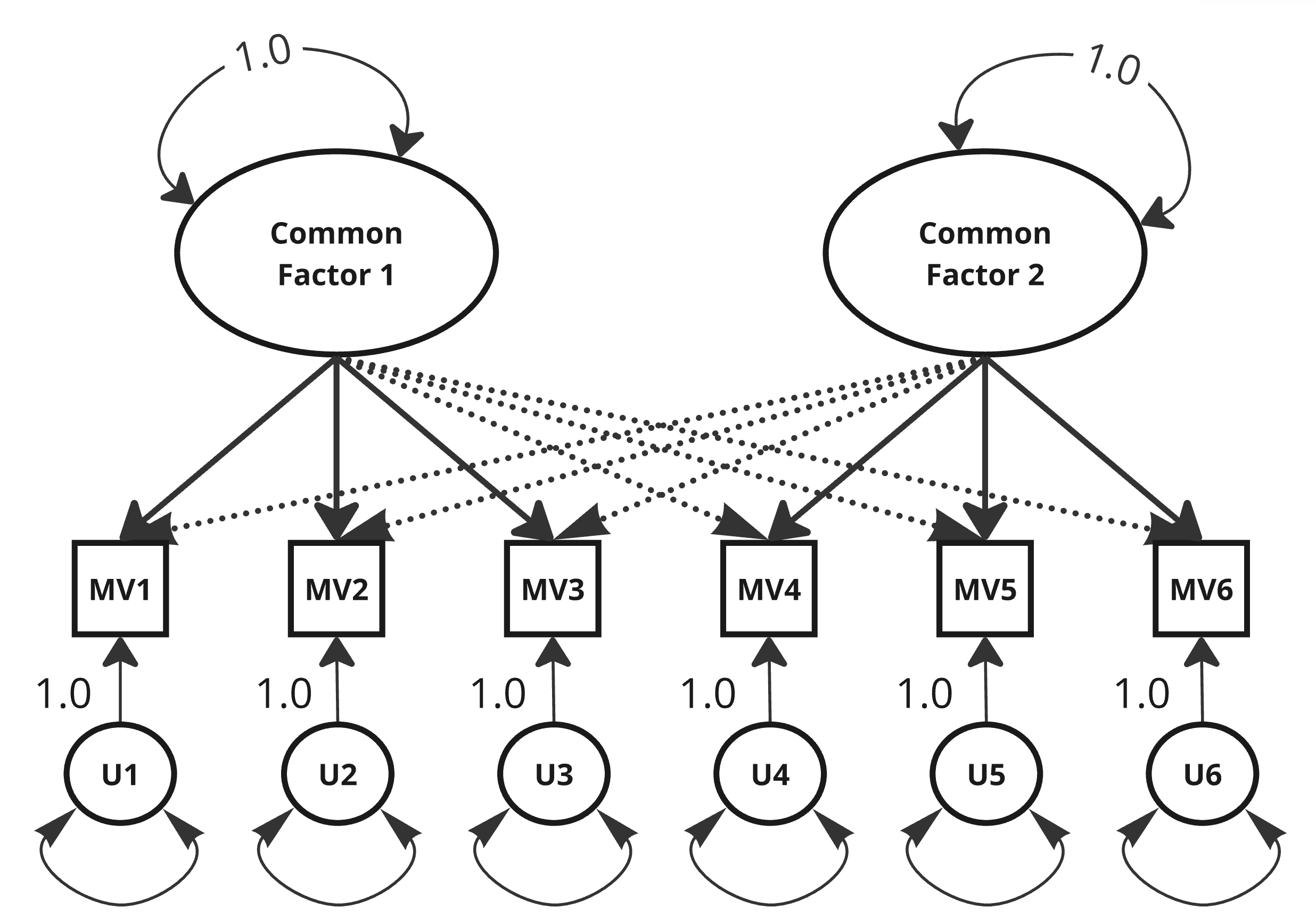
The CFM – Mathematical Representation I
- Fundamental theorem of factor analysis: \(x_{ij}=\lambda_{1j}\eta_{1j} + \lambda_{1j}\eta_{1j} + ... + \lambda_{nj}\eta_{nj} + \varepsilon_{ij}\)
- \(x_{ij}\): value of person \(i\) on MV \(j\)
- \(\lambda_{1j}\): factor loading of factor \(1\) on variable \(j\)
- \(\eta_{1j}\): factor score of person \(i\) on factor \(1\)
- \(\varepsilon_{ij}\): uniqueness (measurement error and value on specific factor) of person \(i\) on MV \(j\)
The CFM – Mathematical Representation II
\[ P=\Lambda\Phi\Lambda^T+\Theta_\delta \]
- \(P\): Population correlation matrix.
- \(\Lambda\): Factor loading matrix (the strength and direction of linear inflence of CFs on MVs).
- \(\Phi\): Factor correlation matrix (also denoted as \(\Psi\); identity matrix in case of orthogonal factors).
- \(\Theta_\delta\): Covariance matrix among unique factors.
The CFM – \(P\)
| MV1 | MV2 | MV3 | MV4 | MV5 | MV6 | |
|---|---|---|---|---|---|---|
| MV1 | 1.00 | |||||
| MV2 | \(\rho_{2,1}\) | 1.00 | ||||
| MV3 | \(\rho_{3,1}\) | \(\rho_{3,2}\) | 1.00 | |||
| MV4 | \(\rho_{4,1}\) | \(\rho_{4,2}\) | \(\rho_{4,3}\) | 1.00 | ||
| MV5 | \(\rho_{5,1}\) | \(\rho_{5,2}\) | \(\rho_{5,3}\) | \(\rho_{5,4}\) | 1.00 | |
| MV6 | \(\rho_{6,1}\) | \(\rho_{6,2}\) | \(\rho_{6,3}\) | \(\rho_{6,4}\) | \(\rho_{6,5}\) | 1.00 |
The CFM – \(\Lambda\), \(\Lambda^T\)
| CF1 | CF2 | |
|---|---|---|
| MV1 | \(\lambda_{1,1}\) | \(\lambda_{1,2}\) |
| MV2 | \(\lambda_{2,1}\) | \(\lambda_{2,2}\) |
| MV3 | \(\lambda_{3,1}\) | \(\lambda_{3,2}\) |
| MV4 | \(\lambda_{4,1}\) | \(\lambda_{4,2}\) |
| MV5 | \(\lambda_{5,1}\) | \(\lambda_{5,2}\) |
| MV6 | \(\lambda_{6,1}\) | \(\lambda_{6,2}\) |
| MV1 | MV2 | MV3 | MV4 | MV5 | MV6 | |
|---|---|---|---|---|---|---|
| CF1 | \(\lambda_{1,1}\) | \(\lambda_{2,1}\) | \(\lambda_{3,1}\) | \(\lambda_{4,1}\) | \(\lambda_{5,1}\) | \(\lambda_{6,1}\) |
| CF2 | \(\lambda_{1,2}\) | \(\lambda_{2,2}\) | \(\lambda_{3,2}\) | \(\lambda_{4,2}\) | \(\lambda_{5,2}\) | \(\lambda_{6,2}\) |
The CFM – \(\Phi\)
| CF1 | CF2 | |
|---|---|---|
| MV1 | 1.00 | |
| MV2 | \(\phi_{2,1}\) | 1.00 |
\(\rightarrow\) When CFs are orthogonal, \(\Phi\) is an identity matrix.
The CFM – \(\Theta_\delta\)
| U1 | U2 | U3 | U4 | U5 | U6 | |
|---|---|---|---|---|---|---|
| U1 | \(\delta_{ 1,1}\) | |||||
| U2 | 0 | \(\delta_{2,2}\) | ||||
| U3 | 0 | 0 | \(\delta_{3,3}\) | |||
| U4 | 0 | 0 | 0 | \(\delta_{4,4}\) | ||
| U5 | 0 | 0 | 0 | 0 | \(\delta_{5,5}\) | |
| U6 | 0 | 0 | 0 | 0 | 0 | \(\delta_{6,6}\) |
Matrix Multiplication
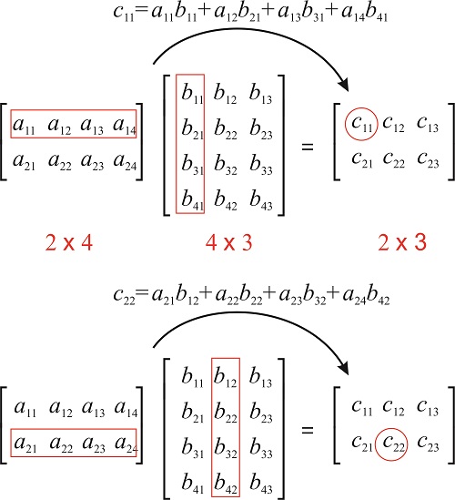
The CFM – Example Calculations
\[ P=\Lambda\Phi\Lambda^T+\Theta_\delta \]
Assuming orthogonal factors:
- \(\rho_{1,1} = 1.00 = \lambda_{1, 1}\lambda_{1, 1} + \lambda_{1, 2}\lambda_{1, 2} + \delta_{1,1} = \lambda_{1, 1}^2 + \lambda_{1, 2}^2 + \delta_{1,1}\)
- \(\rho_{2,1} = \lambda_{2, 1}\lambda_{1, 1} + \lambda_{2, 2}\lambda_{1, 2}\)
Assuming correlated factors:
- \(\rho_{2,1} = (\lambda_{2, 1} + \lambda_{2, 2}\phi_{2,1})\lambda_{1, 1} + (\lambda_{2, 2}\phi_{2,1} + \lambda_{2,2})\lambda_{1, 2}\)
Kinds of Factor Analysis
We look at two kinds of factor analysis:
- Exploratory factor analysis (EFA):
- Also unrestricted factor analysis
- A data-driven approach; use when…
- no (well developed) theory
- newly developed measure
- very large data (cross-validation)
- a large number of competing theories exist
R-packages:{psych},{lavaan},{EFAtools}
- Confirmatory factor analysis (CFA):
- Also restricted factor analysis
- Use when…
- clear theory
- previous EFA conducted
- validated measure
- a couple of competing theories
R-package:{lavaan}
References
![]()
Introduction to Factor Analysis - GSP 2025 - University of Basel